The amount and health of land, including soil quality, for ecological and human use.

Icon

Improve Annual Cropping

Image
Coming Soon
Off
Summary

Farmers on much of the world’s 1.4 billion ha of cropland grow and harvest annual crops – crops like wheat, rice, and soybeans that live for one year or less. After harvest, croplands are often left bare for the rest of the year and sometimes tilled, exposing the soil to wind and rain. This keeps soil carbon levels low and can lead to soil erosion. There are many ways to improve annual cropping to protect or enhance the health of the soil and increase soil organic matter. Project Drawdown’s Improve Annual Cropping solution is a set of practices that protects soils by minimizing plowing (no-till/reduced tillage) and maintaining continuous soil cover (by retaining crop residues or growing cover crops). This increases soil carbon sequestration and reduces nitrous oxide emissions. These techniques are commonly used in conservation agriculture, regenerative, and agro-ecological cropping systems. Other annual cropping practices with desirable climate impacts – including compost application and crop rotations – are omitted here due to lack of data and much smaller scale of adoption. New adoption is estimated from the 2025 level as a baseline which is therefore set to zero.

Description for Social and Search
Improve Annual Cropping is a highly recommended climate solution. It enhances the soil’s ability to store carbon and reduces emissions of nitrous oxide, a potent greenhouse gas.
Overview

The Improve Annual Cropping solution incorporates several practices that minimize soil disturbance and introduce a physical barrier meant to prevent erosion to fragile topsoils. Our definition includes two of the three pillars of conservation agriculture: minimal soil disturbance and permanent soil cover (Kassam et al., 2022).

Minimal Soil Disturbance

Soil organic carbon (SOC) – which originates from decomposed plants – helps soils hold moisture and provides the kinds of chemical bonding that allow nutrients to be stored and exchanged easily with plants. Soil health and productivity depend on microbial decomposition of plant biomass residues, which mobilizes critical nutrients in soil organic matter (SOM) and builds SOC. Conventional tillage inverts soil, buries residues, and breaks down compacted soil aggregates. This process facilitates microbial activity, weed removal, and water infiltration for planting. However, tillage can accelerate CO₂ fluxes as SOC is lost to oxidation and runoff. Mechanical disturbance further exposes deeper soils to the atmosphere, leading to radiative absorption, higher soil temperatures, and catalyzed biological processes – all of which increase oxidation of SOC (Francaviglia et al., 2023).

Reduced tillage limits soil disturbance to support increased microbial activity, moisture retention, and stable temperature at the soil surface. This practice can increase carbon sequestration, at least when combined with cover cropping. These effects are highly contextual, depending on tillage intensity and soil depth as well as the practice type, duration, and timing. Reduced tillage further reduces fossil fuel emissions from on-farm machinery. However, this practice often leads to increased reliance on herbicides for weed control (Francaviglia et al., 2023).

Permanent Soil Cover

Residue retention and cover cropping practices aim to provide permanent plant cover to protect and improve soils. This can improve aggregate stability, water retention, and nutrient cycling. Farmers practicing residue retention leave crop biomass residues on the soil surface to suppress weed growth, improve water infiltration, and reduce evapotranspiration from soils (Francaviglia et al., 2023).

Cover cropping includes growth of spontaneous or seeded plant cover, either during or between established cropping cycles. In addition to SOC, cover cropping can help decrease nitrous oxide emissions and bind nitrogen typically lost via oxidation and leaching. Leguminous cover crops can also fix atmospheric nitrogen, reducing the need for fertilizer. Cover cropping can further be combined with reduced tillage for additive SOC and SOM gains (Blanco-Canqui et al., 2015; Francaviglia et al., 2023).

Improved annual cropping practices can simultaneously reduce GHG emissions and improve SOC stocks. However, there are biological limits to SOC stocks – particularly in mineral soils. Environmental benefits are impermanent and only remain if practices continue long term (Francaviglia et al., 2023).

Abdalla, M., Hastings, A., Cheng, K., Yue, Q., Chadwick, D., Espenberg, M., Truu, J., Rees, R. M., & Smith, P. (2019). A critical review of the impacts of cover crops on nitrogen leaching, net greenhouse gas balance and crop productivity. Global Change Biology, 25(8), 2530–2543. Link to source: https://doi.org/10.1111/gcb.14644 

Arslan, A., McCarthy, N., Lipper, L., Asfaw, S., Cattaneo, A., & Kokwe, M. (2015). Climate smart agriculture? Assessing the adaptation implications in Zambia. Journal of Agricultural Economics66(3), 753-780. Link to source: https://doi.org/10.1111/1477-9552.12107

Bai, X., Huang, Y., Ren, W., Coyne, M., Jacinthe, P.-A., Tao, B., Hui, D., Yang, J., & Matocha, C. (2019). Responses of soil carbon sequestration to climate-smart agriculture practices: A meta-analysis. Global Change Biology25(8), 2591–2606. https://doi.org/10.1111/gcb.14658

Blanco‐Canqui, H., Shaver, T. M., Lindquist, J. L., Shapiro, C. A., Elmore, R. W., Francis, C. A., & Hergert, G. W. (2015). Cover crops and ecosystem services: Insights from studies in temperate soils. Agronomy journal107(6), 2449-2474. Link to source: https://doi.org/10.2134/agronj15.0086

Blanco-Canqui, H., & Francis, C. A. (2016). Building resilient soils through agroecosystem redesign under fluctuating climatic regimes. Journal of Soil and Water Conservation, 71(6), 127A-133A. Link to source: https://doi.org/10.2489/jswc.71.6.127A 

Cai, A., Han, T., Ren, T., Sanderman, J., Rui, Y., Wang, B., Smith, P., Xu, M., & Li, Y. (2022). Declines in soil carbon storage under no tillage can be alleviated in the long run. Geoderma, 425, 116028. Link to source: https://doi.org/10.1016/j.geoderma.2022.116028 

Clapp, J. (2021). Explaining growing glyphosate use: The political economy of herbicide-dependent agriculture. Global Environmental Change67, 102239. Link to source: https://doi.org/10.1016/j.gloenvcha.2021.102239

Cui, Y., Zhang, W., Zhang, Y., Liu, X., Zhang, Y., Zheng, X., Luo, J., & Zou, J. (2024). Effects of no-till on upland crop yield and soil organic carbon: A global meta-analysis. Plant and Soil499(1), 363–377. https://doi.org/10.1007/s11104-022-05854-y

Damania, R., Polasky, S., Ruckelshaus, M., Russ, J., Amann, M., Chaplin-Kramer, R., Gerber, J., Hawthorne, P., Heger, M. P., Mamun, S., Ruta, G., Schmitt, R., Smith, J., Vogl, A., Wagner, F., & Zaveri, E. (2023). Nature's Frontiers: Achieving Sustainability, Efficiency, and Prosperity with Natural Capital. World Bank Publications. Link to source: https://doi.org/10.1596/978-1-4648-1923-0

Francaviglia, R., Almagro, M., & Vicente-Vicente, J. L. (2023). Conservation agriculture and soil organic carbon: Principles, processes, practices and policy options. Soil Systems, 7(1), 17. Link to source: https://doi.org/10.3390/soilsystems7010017 

Griscom, B. W., Adams, J., Ellis, P. W., Houghton, R. A., Lomax, G., Miteva, D. A., Schlesinger, W. H., Shoch, D., Siikamäki, J. V., Smith, P., Woodbury, P., Zganjar, C., Blackman, A., Campari, J., Conant, R. T., Delgado, C., Elias, P., Gopalakrishna, T., Hamsik, M. R., Herrero, M., & Fargione, J. (2017). Natural climate solutions. Proceedings of the National Academy of Sciences114(44), 11645-11650. Link to source: https://doi.org/10.1073/pnas.1710465114

Hassan, M. U., Aamer, M., Mahmood, A., Awan, M. I., Barbanti, L., Seleiman, M. F., Bakhsh, G., Alkharabsheh, H. M., Babur, E., Shao, J., Rasheed, A., & Huang, G. (2022). Management strategies to mitigate N2O emissions in agriculture. Life12(3), 439. Link to source: https://doi.org/10.3390/life12030439

Hu, Q., Thomas, B. W., Powlson, D., Hu, Y., Zhang, Y., Jun, X., Shi, X., & Zhang, Y. (2023). Soil organic carbon fractions in response to soil, environmental and agronomic factors under cover cropping systems: A global meta-analysis. Agriculture, Ecosystems & Environment355, 108591. https://doi.org/10.1016/j.agee.2023.108591

Jat, H. S., Choudhary, K. M., Nandal, D. P., Yadav, A. K., Poonia, T., Singh, Y., Sharma, P. C., & Jat, M. L. (2020). Conservation agriculture-based sustainable intensification of cereal systems leads to energy conservation, higher productivity and farm profitability. Environmental Management, 65(6), 774–786. Link to source: https://doi.org/10.1007/s00267-020-01273-w

Jayaraman, S., Dang, Y. P., Naorem, A., Page, K. L., & Dalal, R. C. (2021). Conservation agriculture as a system to enhance ecosystem services. Agriculture, 11(8), 718. Link to source: https://doi.org/10.3390/agriculture11080718

Kan, Z.-R., Liu, W.-X., Liu, W.-S., Lal, R., Dang, Y. P., Zhao, X., & Zhang, H.-L. (2022). Mechanisms of soil organic carbon stability and its response to no-till: A global synthesis and perspective. Global Change Biology28(3), 693–710. https://doi.org/10.1111/gcb.15968

Kassam, A., Friedrich, T., & Derpsch, R. (2022). Successful experiences and lessons from conservation agriculture worldwide. Agronomy12(4), 769. https://doi.org/10.3390/agronomy12040769

Lal, R., Smith, P., Jungkunst, H. F., Mitsch, W. J., Lehmann, J., Nair, P. K. R., McBratney, A. B., Sá, J. C. D. M., Schneider, J., Zinn, Y. L., Skorupa, A. L. A., Zhang, H.-L., Minasny, B., Srinivasrao, C., & Ravindranath, N. H. (2018). The carbon sequestration potential of terrestrial ecosystems. Journal of Soil and Water Conservation73(6), 145A-152A. Link to source: https://doi.org/10.2489/jswc.73.6.145A

Lessmann, M., Ros, G. H., Young, M. D., & de Vries, W. (2022). Global variation in soil carbon sequestration potential through improved cropland management. Global Change Biology28(3), 1162–1177. https://doi.org/10.1111/gcb.15954

Luo, Z., Wang, E., & Sun, O. J. (2010). Can no-tillage stimulate carbon sequestration in agricultural soils? A meta-analysis of paired experiments. Agriculture, Ecosystems & Environment139(1), 224–231. https://doi.org/10.1016/j.agee.2010.08.006

Martínez-Mena, M., Carrillo-López, E., Boix-Fayos, C., Almagro, M., García Franco, N., Díaz-Pereira, E., Montoya, I., & De Vente, J. (2020). Long-term effectiveness of sustainable land management practices to control runoff, soil erosion, and nutrient loss and the role of rainfall intensity in Mediterranean rainfed agroecosystems. CATENA, 187, 104352. Link to source: https://doi.org/10.1016/j.catena.2019.104352

Moukanni, N., Brewer, K. M., Gaudin, A. C. M., & O’Geen, A. T. (2022). Optimizing carbon sequestration through cover cropping in Mediterranean agroecosystems: Synthesis of mechanisms and implications for management. Frontiers in Agronomy, 4, 844166. Link to source: https://doi.org/10.3389/fagro.2022.844166 

Mrabet, R., Singh, A., Sharma, T., Kassam, A., Friedrich, T., Basch, G., Moussadek, R., & Gonzalez-Sanchez, E. (2023). Conservation Agriculture: Climate Proof and Nature Positive Approach. In G. Ondrasek & L. Zhang (Eds.), Resource management in agroecosystems. IntechOpen. Link to source: https://doi.org/10.5772/intechopen.108890

Nyagumbo, I., Mupangwa, W., Chipindu, L., Rusinamhodzi, L., & Craufurd, P. (2020). A regional synthesis of seven-year maize yield responses to conservation agriculture technologies in Eastern and Southern Africa. Agriculture, Ecosystems & Environment, 295, 106898. Link to source: https://doi.org/10.1016/j.agee.2020.106898

Ogle, S. M., Alsaker, C., Baldock, J., Bernoux, M., Breidt, F. J., McConkey, B., Regina, K., & Vazquez-Amabile, G. G. (2019). Climate and Soil Characteristics Determine Where No-Till Management Can Store Carbon in Soils and Mitigate Greenhouse Gas Emissions. Scientific Reports9(1), 11665. https://doi.org/10.1038/s41598-019-47861-7

Paustian, K., Larson, E., Kent, J., Marx, E., & Swan, A. (2019). Soil C Sequestration as a Biological Negative Emission Strategy. Frontiers in Climate, 1, 8. Link to source: https://doi.org/10.3389/fclim.2019.00008 

Pittelkow, C. M., Liang, X., Linquist, B. A., van Groenigen, K. J., Lee, J., Lundy, M. E., van Gestel, N., Six, J., Venterea, R. T., & van Kessel, C. (2015). Productivity limits and potentials of the principles of conservation agriculture. Nature, 51, 365–368. https://doi.org/10.1038/nature13809

Poeplau, C., & Don, A. (2015). Carbon sequestration in agricultural soils via cultivation of cover crops–A meta-analysis. Agriculture, Ecosystems & Environment200, 33–41. Link to source: https://doi.org/10.1016/j.agee.2014.10.024

Powlson, D. S., Stirling, C. M., Jat, M. L., Gerard, B. G., Palm, C. A., Sanchez, P. A., & Cassman, K. G. (2014). Limited potential of no-till agriculture for climate change mitigation. Nature Climate Change4(8), 678–683. https://doi.org/10.1038/nclimate2292

Prestele, R., Hirsch, A. L., Davin, E. L., Seneviratne, S. I., & Verburg, P. H. (2018). A spatially explicit representation of conservation agriculture for application in global change studies. Global Change Biology24(9), 4038–4053. https://doi.org/10.1111/gcb.14307

Project Drawdown (2020) Farming Our Way Out of the Climate Crisis. Project Drawdown. https://drawdown.org/publications/farming-our-way-out-of-the-climate-crisis

Quintarelli, V., Radicetti, E., Allevato, E., Stazi, S. R., Haider, G., Abideen, Z., Bibi, S., Jamal, A., & Mancinelli, R. (2022). Cover crops for sustainable cropping systems: A review. Agriculture12(12), 2076. Link to source: https://doi.org/10.3390/agriculture12122076

Searchinger, T., R. Waite, C. Hanson, and J. Ranganathan. (2019). World Resources Report: Creating a Sustainable Food Future. Washington, DC: World Resources Institute. Link to source: https://research.wri.org/sites/default/files/2019-07/WRR_Food_Full_Report_0.pdf

Stavi, I., Bel, G., & Zaady, E. (2016). Soil functions and ecosystem services in conventional, conservation, and integrated agricultural systems. A review. Agronomy for Sustainable Development, 36(2), 32. Link to source: https://doi.org/10.1007/s13593-016-0368-8

Su, Y., Gabrielle, B., Beillouin, D., & Makowski, D. (2021). High probability of yield gain through conservation agriculture in dry regions for major staple crops. Scientific Reports, 11(1), 3344. Link to source: https://doi.org/10.1038/s41598-021-82375-1

Sun, W., Canadell, J. G., Yu, L., Yu, L., Zhang, W., Smith, P., Fischer, T., & Huang, Y. (2020). Climate drives global soil carbon sequestration and crop yield changes under conservation agriculture. Global Change Biology, 26(6), 3325–3335. Link to source: https://doi.org/10.1111/gcb.15001 

Tambo, J. A., & Mockshell, J. (2018). Differential impacts of conservation agriculture technology options on household income in sub-Saharan Africa. Ecological Economics, 151, 95–105. Link to source: https://doi.org/10.1016/j.ecolecon.2018.05.005

Tiefenbacher, A., Sandén, T., Haslmayr, H.-P., Miloczki, J., Wenzel, W., & Spiegel, H. (2021). Optimizing carbon sequestration in croplands: A synthesis. Agronomy, 11(5), 882. Link to source: https://doi.org/10.3390/agronomy11050882

Toensmeier, E. (2016). The Carbon Farming Solution: A Global Toolkit of Perennial Crops and Regenerative Agriculture Practices for Climate Change Mitigation and Food Security. Green Publishing. Link to source: https://www.chelseagreen.com/product/the-carbon-farming-solution/?srsltid=AfmBOoqsMoY569HfsXOdBsRguOzsDLlRZKOnyM4nyKwZoIALvPoohZlq 

Vendig, I., Guzman, A., De La Cerda, G., Esquivel, K., Mayer, A. C., Ponisio, L., & Bowles, T. M. (2023). Quantifying direct yield benefits of soil carbon increases from cover cropping. Nature Sustainability6(9), 1125–1134. https://doi.org/10.1038/s41893-023-01131-7

WCCA (2021). The future of farming: Profitable and sustainable farming with conservation agriculture. 8th World Congress on Conservation Agriculture, Vern Switzerland. Link to source: https://ecaf.org/8wcca

Wooliver, R., & Jagadamma, S. (2023). Response of soil organic carbon fractions to cover cropping: A meta-analysis of agroecosystems. Agriculture, Ecosystems & Environment351, 108497. https://doi.org/10.1016/j.agee.2023.108497

Xing, Y., & Wang, X. (2024). Impact of agricultural activities on climate change: a review of greenhouse gas emission patterns in field crop systems. Plants13(16), 2285. Link to source: https://doi.org/10.3390/plants13162285

Credits

Lead Fellows

  • Avery Driscoll

  • Erika Luna

  • Megan Matthews, Ph.D.

  • Eric Toensmeier

  • Aishwarya Venkat, Ph.D.

Contributors

  • Ruthie Burrows, Ph.D.

  • James Gerber, Ph.D.

  • Yusuf Jameel, Ph.D.

  • Daniel Jasper

  • Alex Sweeney

Internal Reviewers

  • Aiyana Bodi

  • Emily Cassidy, Ph.D.

  • James Gerber, Ph.D.

  • Hannah Henkin

  • Zoltan Nagy, Ph.D.

  • Ted Otte

  • Paul C. West, Ph.D.

Effectiveness

Based on seven reviews and meta-analyses, which collectively analyzed over 500 studies, we estimate that this solution’s SOC sequestration potential is 1.28 t CO₂‑eq/ha/yr. This is limited to the topsoil (>30 cm), with minimal effects at deeper levels (Sun et al., 2020; Tiefenbacher et al., 2021). Moreover, carbon sequestration potential is not constant over time. The first two decades show the highest increase, followed by an equilibrium or SOC saturation (Cai, 2022; Sun et al., 2020).

The effectiveness of the Improve Annual Cropping solution heavily depends on local geographic conditions (e.g., soil properties, climate), crop management practices, cover crop biomass, cover crop types, and the duration of annual cropping production – with effects typically better assessed in the long term (Abdalla et al., 2019; Francaviglia et al., 2023; Moukanni et al., 2022; Paustian et al., 2019).

Based on reviewed literature (three papers, 18 studies), we estimated that improved annual cropping can potentially reduce nitrous oxide emissions by 0.51 t CO₂‑eq/ha/yr (Table 1). Cover crops can increase direct nitrous oxide emissions by stimulating microbial activity, but – compared with conventional cropping – lower indirect emissions allow for reduced net nitrous oxide emissions from cropland (Abdalla et al., 2019). 

Nitrogen fertilizers drive direct nitrous oxide emissions, so genetic optimization of cover crops to increase nitrogen-use efficiencies and decrease nitrogen leaching could further improve mitigation of direct nitrous oxide emissions (Abdalla et al., 2019). 

left_text_column_width

Table 1. Effectiveness at reducing emissions and removing carbon.

Unit: t CO₂‑eq/ha/yr, 100-yr basis

25th percentile 0.29
median (50th percentile) 0.51
75th percentile 0.80

Unit: t CO₂‑eq/ha/yr, 100-yr basis

25th percentile 0.58
median (50th percentile) 1.28
75th percentile 1.72

Unit: t CO₂‑eq/ha/yr, 100-yr basis

25th percentile 0.87
median (50th percentile) 1.79
75th percentile 2.52
Left Text Column Width
Cost

Because baseline (conventional) annual cropping systems are already extensive and well established, we assume there is no cost to establish new baseline cropland. In the absence of global datasets on costs and revenues of cropping systems, we used data on the global average profit per ha of cropland from Damania et al. (2023) to create a weighted average profit of US$76.86/ha/yr.

Based on 13 data points (of which seven were from the United States), the median establishment cost of the Improve Annual Cropping solution is $329.78/ha. Nine data points (three from the United States) provided a median increase in profitability of US$86.01/ha/yr. 

The net net cost of the Improve Annual Cropping solution is US$86.01. The cost per t CO₂‑eq is US$47.80 (Table 2).

left_text_column_width

Table 2. Cost per unit climate impact.

Unit: 2023 US$/t CO₂‑eq, 100-yr basis

median 47.80
Left Text Column Width
Learning Curve

We found limited information on this solution’s learning curve. A survey of farmers in Zambia found a reluctance to avoid tilling soils because of the increased need for weeding or herbicides and because crop residues may need to be used for livestock feed (Arslan et al., 2015; Searchinger et al., 2019).

left_text_column_width
Speed of Action

Speed of action refers to how quickly a climate solution physically affects the atmosphere after it is deployed. This is different from speed of deployment, which is the pace at which solutions are adopted.

At Project Drawdown, we define the speed of action for each climate solution as emergency brake, gradual, or delayed.

Improve Annual Cropping is a DELAYED climate solution. It works more slowly than gradual or emergency brake solutions. Delayed solutions can be robust climate solutions, but it’s important to recognize that they may not realize their full potential for some time.

left_text_column_width
Caveats

As with other biosequestration solutions, carbon stored in soils via improved annual cropping is not permanent. It can be lost quickly through a return to conventional agriculture practices like plowing, and/or through a regional shift to a drier climate or other human- or climate change–driven disturbances. Carbon sequestration also only continues for a limited time, estimated at 20–50 years (Lal et al., 2018)).

left_text_column_width
Current Adoption

Kassam et al. (2022) provided regional adoption from 2008–2019. We used a linear forecast to project 2025 adoption. This provided a figure of 267.4 Mha in 2025 (Table 3). Note that in Solution Basics in the dashboard we set current adoption at zero. This is a conservative assumption to avoid counting carbon sequestration from land that has already ceased to sequester net carbon due to saturation, which takes place after 20–50 years (Lal et al., 2018).

left_text_column_width

Table 3. Current (2025) adoption level.

Unit: Mha of improved annual cropping

Drawdown estimate 267.4
Left Text Column Width
Adoption Trend

Between 2008–2009 and 2018–2019 (the most recent data available), the cropland area under improved annual cropping practices nearly doubled globally, increasing from 10.6 Mha to 20.5 Mha at an average rate of 1.0 Mha/yr (Kassam et al., 2022), equivalent to a 9.2% annual increase in area relative to 2008–2009 levels. Adoption slowed slightly in the latter half of the decade, with an average increase of 0.8 Mha/yr between 2015–2016 and 2018–2019, equivalent to 4.6% annual increase in area relative to 2015–2016 levels, as shown in Table 4.

left_text_column_width

Table 4. 2008–2009 to 2018–2019 adoption trend.

Unit: Mha adopted/yr

mean 9.99
Left Text Column Width
Adoption Ceiling

Griscom et al. (2017) estimate that 800 Mha of global cropland are suitable – but not yet used for – cover cropping, in addition to 168 Mha already in cover crops (Popelau and Don, 2015). We update the 168 Mha in cover crops to 267 Mha based on Kassam (2022). Griscom et al.’s estimate is based on their analysis that much cropland is unsuitable because it already is used to produce crops during seasons in which cover crops would be grown. Their estimate thus provides a maximum technical potential of 1,067 Mha  by adding 800 Mha of remaining potential to the 267.4 Mha of current adoption (Table 5). 

left_text_column_width

Table 5. Adoption ceiling.

Unit: Mha

Adoption ceiling 1,067
Left Text Column Width
Achievable Adoption

The 8th World Congress on Conservation Agriculture (8WCCA) set a goal to achieve adoption of improved annual cropping on 50% of available cropland by 2050 (WCCA 2021). That provides an Achievable – High of 700 Mha – though this is not a biophysical limit. 

We used the 2008–2019 data from Kassam (2022) to calculate average annual regional growth rates. From these we selected the 25th percentile as our low achievable level (Table 6).

left_text_column_width

Table 6. Range of achievable adoption levels.

Unit: Mha

Current Adoption 267.4
Achievable – Low 331.7
Achievable – High 700.0
Adoption Ceiling 1,067

Unit: Mha installed

Current Adoption 0.00
Achievable – Low 64.2
Achievable – High 432.6
Adoption Ceiling 868.6
Left Text Column Width

Carbon sequestration continues only for a period of decades; because adoption of improved annual cropping was already underway in the 1970s (Kassam et al., 2022), we could not assume that previously adopted hectares continue to sequester carbon indefinitely. Much of the current adoption of improved annual cropping has been in place for decades and sequestration in some of this land has presumably already slowed down to almost zero. We apply an adoption adjustment factor of 0.5 to current adoption (see methodology) to reflect that an estimated half of current adoption is no longer sequestering significant carbon, yet there is substantial new adoption within the last 20-50 years.

For new adoption, the calculation is effectiveness * new adoption = climate impact.

For calculating impact of current adoption, the calculation is the sum of and where:

a:  for carbon sequestration, the calculation is effectiveness * 0.5 * current adoption = climate impact, and

b: for nitrous oxide reduction, the calculation is effectiveness * current adoption = climate impact.

Climate impacts shown in Table 6 are the sum of current and new adoption impacts. Combined effect is 0.31 Gt CO2-eq/yr for current adoption, 0.43 for Achievable – Low, 1.09 for Achievable – High, and 1.87 for our Adoption Ceiling.

left_text_column_width

Table 8. Climate impact at different levels of adoption.

Unit: Gt CO₂ ‑eq/yr, 100-yr basis

Current Adoption 0.14
Achievable – Low 0.17
Achievable – High 0.36
Adoption Ceiling 0.58

(from nitrous oxide)

Unit: Gt CO₂ ‑eq/yr, 100-yr basis

Current Adoption 0.17
Achievable – Low 0.25
Achievable – High 0.73
Adoption Ceiling 1.29

(from SOC)

Unit: Gt CO₂ ‑eq/yr, 100-yr basis

Current Adoption 0.31
Achievable – Low 0.43
Achievable – High 1.09
Adoption Ceiling 1.87
Left Text Column Width
Additional Benefits

Extreme Weather Events

The soil and water benefits of this solution can lead to agricultural systems that are more resilient to extreme weather events (Mrabet et al., 2023). These agricultural systems have improved uptake, conservation, and use of water, so they are more likely to successfully cope and adapt to drought, dry conditions, and other adverse weather events (Su et al., 2021). Additionally, more sustained year-round plant cover can increase the capacity of cropping systems to adapt to high temperatures and extreme rainfall (Blanco-Canqui & Francis, 2016; Martínez-Mena et al., 2020).

Droughts

Increased organic matter due to improved annual cropping increases soil water holding capacity. This increases drought resilience (Su et al., 2021). 

Income and Work

Conservation agriculture practices can reduce costs on fuel, fertilizer, and pesticides (Stavi et al., 2016). The highest revenues from improved annual cropping are often found in drier climates. Tambo et al. (2018) found when smallholder farmers in sub-Saharan Africa jointly employed the three aspects of conservation agriculture – reduced tillage, cover crops, and crop rotation – households and individuals saw the largest income gains. Nyagumbo et al. (2020) found that smallholder farms in sub-Saharan Africa using conservation agriculture had the highest returns on crop yields when rainfall was low. 

Food Security

Improved annual cropping can improve food security by increasing the amount and the stability of crop yields. A meta-analysis of studies of South Asian cropping systems found that those following conservation agriculture methods had 5.8% higher mean yield than cropping systems with more conventional agriculture practices (Jat et al., 2020). Evidence supports that conservation agriculture practices especially improve yields in water scarce areas (Su et al., 2021). Nyagumbo et al. (2020) found that smallholder farmers in sub-Saharan Africa experienced reduced yield variability when using conservation agriculture practices.

Nature Protection

Improved annual cropping can increase biodiversity below and above soils (Mrabet et al., 2023). Increased vegetation cover improves habitats for arthropods, which help with pest and pathogen management (Stavi et al., 2016).

Land Resources

Improved annual cropping methods can lead to improved soil health through increased stability of soil structure, increased soil nutrients, and improved soil water storage (Francaviglia et al., 2023). This can reduce soil degradation and erosion (Mrabet et al., 2023). Additionally, more soil organic matter can lead to additional microbial growth and nutrient availability for crops (Blanco-Canqui & Francis, 2016). 

Water Quality

Runoff of soil and other agrochemicals can be minimized through conservation agricultural practices, reducing the amount of nitrate and phosphorus that leach into waterways and contribute to algal blooms and eutrophication (Jayaraman et al., 2021). Abdalla et al. (2019) found that cover crops reduced nitrogen leaching.

left_text_column_width
Risks

Herbicides – in place of tillage – are used in many but not all no-till cropping systems to kill (terminate) the cover crop. The large-scale use of herbicides in improved annual cropping systems can produce a range of environmental and human health consequences. Agricultural impacts can include development of herbicide-resistant weeds (Clapp, 2021). 

If cover crops are not fully terminated before establishing the main crop, there is a risk that cover crops can compete with the main crop (Quintarelli et al., 2022). 

left_text_column_width
Interactions with Other Solutions

Improved annual cropping has competing interactions with several other solutions related to shifting annual practices. For each of these other solutions, the Improve Annual Cropping solution can reduce the area on which the solution can be applied or the nutrient excess available for improved management. 

left_text_column_width

COMPETING

In no-till systems, cover crops are typically terminated with herbicides, often preventing incorporation of trees depending on the type of herbicide used.

left_text_column_width

Land managed under the Improve Annual Cropping solution is not available for perennial crops.

left_text_column_width

Improved annual cropping typically reduces fertilizer demand, reducing the scale of climate impact under improved nutrient management. 

left_text_column_width

Our definition of improved annual cropping requires residue retention, limiting the additional area available for deployment of reduced burning.

left_text_column_width
Dashboard

Solution Basics

ha cropland

t CO₂-eq (100-yr)/unit/yr
00.881.8
units
Current 2.674×10⁸ 03.317×10⁸7×10⁸
Achievable (Low to High)

Climate Impact

Gt CO₂-eq (100-yr)/yr
Current 0.31 0.431.09
US$ per t CO₂-eq
48
Delayed

CO₂, N₂O

Trade-offs

Some studies have found that conservation tillage without cover crops can reduce soil carbon stocks in deeper soil layers. They caution against overreliance on no-till as a sequestration solution in the absence of cover cropping. Reduced tillage should be combined with cover crops to ensure carbon sequestration (Luo et al., 2010; Ogle et al., 2019; Powlson et al., 2014).

left_text_column_width
t CO2-eq/ha
0≥ 400

Thousands of years of agricultural land use have removed nearly 500 Gt CO2-eq from soils

Agriculture has altered the soil carbon balance around the world, resulting in changes (mostly losses) of soil carbon. Much of the nearly 500 Gt CO2-eq lost in the last 12,000 years is now in the atmosphere in the form of CO2.

Sanderman, J. et al. (2017). The soil carbon debt of 12,000 years of human land use [Data set]. PNAS 114(36): 9575–9580. Link to source: https://doi.org/10.1073/pnas.1706103114

Maps Introduction

Adoption of this solution varies substantially across the globe. Currently, improved annual cropping practices are widely implemented in Australia and New Zealand (74% of annual cropland) and Central and South America (69%), with intermediate adoption in North America (34%) and low adoption in Asia, Europe, and Africa (1–5%) (Kassam et al., 2022), though estimates vary (see also Prestele et al., 2018). Future expansion of this solution is most promising in Asia, Africa, and Europe, where adoption has increased in recent years. Large areas of croplands are still available for implementation in these regions, whereas Australia, New Zealand, and Central and South America may be reaching a saturation point, and these practices may be less suitable for the relatively small area of remaining croplands.

The carbon sequestration effectiveness of this solution also varies across space. Drivers of soil carbon sequestration rates are complex and interactive, with climate, initial soil carbon content, soil texture, soil chemical properties (such as pH), and other land management practices all influencing the effectiveness of adopting this solution. Very broadly, the carbon sequestration potential of improved annual cropping tends to be two to three times higher in warm areas than cool areas (Bai et al., 2019; Cui et al., 2024; Lessmann et al., 2022). Warm and humid conditions enable vigorous cover crop growth, providing additional carbon inputs into soils. Complicating patterns of effectiveness, however, arid regions often experience increased crop yields following adoption of this solution whereas humid regions are more likely to experience yield losses (Pittelkow et al., 2015). Yield losses may reduce adoption in humid areas and can lead to cropland expansion to compensate for lower production. 

Uptake of this solution may be constrained by spatial variation in places where cover cropping is suitable. In areas with double or triple cropping, there may not be an adequate interval for growth of a cover crop between harvests. In areas with an extended dry season, there may be inadequate moisture to grow a cover crop.

Action Word
Improve
Solution Title
Annual Cropping
Classification
Highly Recommended
Lawmakers and Policymakers
  • Provide local and regional institutional guidance for improving annual cropping that adapts to the socio-environmental context.
  • Integrate soil protection into national climate mitigation and adaptation plans.
  • Remove financial incentives, such as subsidies, for unsustainable practices and replace them with financial incentives for carbon sequestration practices.
  • Place taxes or fines on emissions and related farm inputs (such as nitrogen fertilizers).
  • Reform international agricultural trade, remove subsidies for emissions-intensive agriculture, and support climate-friendly practices.
  • Strengthen and support land tenure for smallholder farmers.
  • Mandate insurance schemes that allow farmers to use cover crops and reduce tillage.
  • Support, protect, and promote traditional and Indigenous knowledge of land management practices.
  • Set standards for measuring, monitoring, and verifying impacts on SOC accounting for varying socio-environmental conditions.
  • Develop economic budgets for farmers to adopt these practices.
  • Invest in or expand extension services to educate farmers and other stakeholders on the economic and environmental benefits of improved annual cropping.
  • Create, support, or join education campaigns and/or public-private partnerships that facilitate stakeholder discussions.
Practitioners
  • Implement no-till practices and use cover crops.
  • Utilize or advocate for financial assistance and tax breaks for farmers to use improved annual cropping techniques.
  • Adjust the timing and dates of the planting and termination of the cover crops in order to avoid competition for resources with the primary crop.
  • Find opportunities to reduce initial operation costs of no-tillage and cover crops, such as selling cover crops as forage or grazing.
  • Take advantage of education programs, support groups, and extension services focused on improved annual cropping methods.
  • Create, support, or join stakeholder discussions, especially around standardized monitoring frameworks, ROI, and climate benefits.
Business Leaders
  • Source from producers implementing improved annual cropping practices, create programs that directly engage and educate farmers, and promote inspiring case studies with the industry and wider public.
  • Create sustainability goals and supplier requirements that incorporate this solution and offer pricing incentives for compliant suppliers.
  • Invest in companies that utilize improved annual cropping techniques or produce the necessary inputs.
  • Promote and develop markets for products that employ improved annual cropping techniques and educate consumers about the importance of the practice.
  • Stay abreast of recent scientific findings and use third-party verification to monitor sourcing practices.
  • Offer financial services – including low-interest loans, micro-financing, and grants – to support low-carbon agriculture (e.g., sustainable land management systems).
  • Support high-integrity carbon markets, institutions, rules, and norms to cultivate the demand for high-quality carbon credits.
  • Create, support, or join education campaigns and/or public-private partnerships that facilitate stakeholder discussions, especially around standardized monitoring frameworks, ROI, and climate benefits.
Nonprofit Leaders
  • Start model farms to demonstrate techniques, conduct experiments, and educate local farmers.
  • Conduct and share research on improving annual cropping techniques and local policy options.
  • Advocate to policymakers for improving annual cropping techniques, incentives, and regulations.
  • Educate farmers on sustainable means of agriculture and support implementation.
  • Help integrate improved annual cropping practices as part of the broader climate agenda.
  • Engage with businesses to encourage corporate responsibility and/or monitor soil health.
  • Offer resources and training in financial planning and yield risk management to farmers adopting improved annual cropping approaches.
  • Partner with research institutions and businesses to co-develop and distribute region-specific best practices.
  • Create, support, or join stakeholder discussions, especially around standardized monitoring frameworks, ROI, and climate benefits.
Investors
  • Integrate science-based due diligence on improved annual cropping techniques and soil health measures into all farming and agritech investments.
  • Encourage companies in your investment portfolio to adopt improved annual cropping practices.
  • Offer access to capital, such as low-interest loans, micro-financing, and grants to improve annual cropping.
  • Invest in companies developing technologies that improve annual cropping, such as soil management equipment and related software.
  • Create, support, or join stakeholder discussions, especially around standardized monitoring frameworks, ROI, and climate benefits.
Philanthropists and International Aid Agencies
  • Start model farms to demonstrate techniques, conduct experiments, and educate local farmers.
  • Offer access to capital, such as low-interest loans, micro-financing, and grants to support improving annual cropping, (e.g., traditional land management).
  • Conduct and share research on improved annual cropping techniques and local policy options.
  • Advocate to policymakers for improved annual cropping techniques, incentives, and regulations.
  • Educate farmers on traditional means of agriculture and support implementation.
  • Help integrate improved annual cropping practices as part of the broader climate agenda.
  • Engage with businesses to encourage corporate responsibility and/or monitor soil health.
  • Offer resources and training in financial planning and yield risk management to farmers adopting improved annual cropping approaches.
  • Partner with research institutions and businesses to co-develop and distribute region-specific best practices.
  • Create, support, or join stakeholder discussions, especially around standardized monitoring frameworks, ROI, and climate benefits.
  • Invest in companies developing technologies that improve annual cropping, such as soil management equipment and related software.
Thought Leaders
  • Start model farms to demonstrate techniques, conduct experiments, and educate local farmers.
  • Conduct and share research on improved annual cropping techniques and local policy options.
  • Advocate to policymakers for improved annual cropping techniques, incentives, and regulations.
  • Educate farmers on traditional means of agriculture and support implementation.
  • Engage with businesses to encourage corporate responsibility and/or monitor soil health.
  • Research the regional impacts of cover crops on SOC and SOM and publish the data.
  • Partner with research institutions and businesses to co-develop and distribute region-specific best practices.
  • Create, support, or join stakeholder discussions, especially around standardized monitoring frameworks, ROI, and climate benefits.
  • Work with farmers and other private organizations to improve data collection on uptake of improved annual cropping techniques, effectiveness, and regional best practices.
Technologists and Researchers
  • Help develop standards for measuring, monitoring, and verifying impacts on SOC accounting for varying socio-environmental conditions.
  • Research the regional impacts of cover crops (particularly outside the United States) on SOC and SOM, and publish the data.
  • Create tracking and monitoring software to support farmers' decision-making.
  • Research the application of AI and robotics for crop rotation.
  • Improve data and analytics to monitor soil and water quality, assist farmers, support policymaking, and assess the impacts of policies.
  • Develop education and training applications to improve annual cropping techniques and provide real-time feedback.
Communities, Households, and Individuals
  • Participate in urban agriculture or community gardening programs that implement these practices.
  • Engage with businesses to encourage corporate responsibility and/or monitor soil health.
  • Work with farmers and other private organizations to improve data collection on uptake of improved annual cropping techniques, effectiveness, and regional best practices.
  • Advocate to policymakers for improved annual cropping techniques, incentives, and regulations.
  • Start model farms to demonstrate techniques, conduct experiments, and educate local farmers.
  • Educate farmers on traditional means of agriculture and support implementation.
  • Create, support, or join stakeholder discussions, especially around standardized monitoring frameworks, ROI, and climate benefits.
Evidence Base

Consensus of effectiveness of cover cropping for sequestering carbon: 

The impacts of improved annual cropping practices on soil carbon sequestration have been extensively studied, and there is high consensus that adoption of cover crops can increase carbon sequestration in soils. However, estimates of how much carbon can be sequestered vary substantially, and sequestration rates are strongly influenced by factors such as climate, soil properties, time since adoption, and how the practices are implemented.

The carbon sequestration benefits of cover cropping are well established. They have been documented in reviews and meta-analyses including Hu et al. (2023) and Vendig et al. (2023). 

Consensus of effectiveness of reduced tillage for sequestering carbon: Mixed

Relative to conventional tillage, estimates of soil carbon gains in shallow soils under no-till management include average increases of 5–20% (Bai et al., 2019; Cui et al., 2024; Kan et al., 2022). Lessmann et al. (2022) estimated that use of no-till is associated with an average annual increase in carbon sequestration of 0.88 t CO₂‑eq /ha/yr relative to high-intensity tillage. 

Nitrous oxide reduction: Mixed

Consensus on nitrous oxide reductions from improved annual cropping is mixed. Several reviews have demonstrated a modest reduction in nitrous oxide from cover cropping (Abdalla et al., 2019; Xing & Wang, 2024). Reduced tillage can result in either increased or decreased nitrous oxide emissions (Hassan et al., 2022). 

The results presented in this document summarize findings from 10 reviews and meta-analyses reflecting current evidence at the global scale. Nonetheless, not all countries are represented. We recognize this limited geographic scope creates bias, and hope this work inspires research and data sharing on this topic in underrepresented regions.

left_text_column_width
Updated Date

Improve Rice Production

Image
Image
Rice field
Coming Soon
Off
Summary

Rice production is a significant source of methane emissions and a minor source of nitrous oxide emissions. Most rice production occurs in flooded fields called paddies, where anaerobic conditions trigger high levels of methane production. This solution includes two related practices that each reduce emissions from paddy rice production: noncontinuous flooding and nutrient management. Noncontinuous flooding is a water management technique that reduces the amount of time rice paddy soils spend fully saturated, thereby reducing methane. Unfortunately, noncontinuous flooding increases nitrous oxide emissions. Nutrient management helps to address this challenge by controlling the timing, amount, and type of fertilization to maximize plant uptake and minimize nitrous oxide emissions.

Description for Social and Search
Improve Rice Production is a Highly Recommended climate solution. It reduces emissions of methane and nitrous oxide, two potent greenhouse gases, by converting rice paddies from continuous flooding to noncontinuous flooding and improving nutrient management.
Overview

Rice is a staple crop of critical importance, occupying 11% of global cropland (FAOstat 2025). Rice production has higher GHG emissions than most crop production, accounting for 9% of all anthropogenic methane and 10% of cropland nitrous oxide (Wang et al., 2020). Nabuurs et al. (2022) found methane emissions from global rice production to be 0.8–1.0 Gt CO₂‑eq/yr and growing 0.4% annually.

Rice paddy systems are fields with berms and plumbing to permit the flooding of rice for the production periods, which helps with weed and pest control (rice thrives in flooded conditions, though it does not require them). Paddy rice is the main source of methane from rice production. Upland rice is grown outside of paddies and does not produce significant methane emissions, so we excluded it from this analysis. Irrigated paddies are provided with irrigation water, while rain-fed paddies are only filled by rainfall and runoff (Raffa, 2021). For this analysis, we considered both irrigated and rain-fed paddies.

Methane Reduction

Flooded rice paddies encourage the production of methane by microbes. Conventional paddy rice production uses continuous flooding, in which the paddy is flooded for the full rice production period. Several approaches can reduce methane, with the most widespread being noncontinuous flooding. This is a collection of practices (such as alternate wetting and drying) that drain the fields one or more times during the rice production period. As a result, the paddy spends less time in its methane-producing state. This can be done without reducing rice yields in many, but not all, cases, and also significantly reduces irrigation water use (Bo et al., 2022). Impacts on yields depend on soils, climate, and other variables (Cheng et al., 2022). 

Nitrous Oxide Reduction

A major drawback to noncontinuous flooding is that it increases nitrous oxide emissions from fertilizer compared to continuous flooding. High nitrogen levels in flooded paddies encourage the growth of bacteria that produce methane, reduce the natural breakdown of methane, and facilitate emissions of nitrous oxide to the atmosphere (Li et al., 2024). The effect is small compared to the mitigated emissions from methane reduction (Jiang et al., 2019), but remains serious. Use of nutrient management techniques, such as controlling fertilizer amount, type (e.g., controlled-release urea), timing, and application techniques (e.g., deep fertilization), can reduce these emissions. This is in part because nitrogen fertilizers are often overapplied, leaving room to increase efficiency without reducing rice yields (Hergoualc’h et al., 2019; Li et al., 2024). 

Other Promising Practices

Other practices also show potential but were not included in our analysis. These include the application of biochar to rice paddies and the use of rice cultivars that produce fewer emissions (Qian et al., 2023). Other approaches include saturated soil culture, System of Rice Intensification (“SRI”), ground-cover systems, raised beds, and improved irrigation and paddy infrastructure (Surendran et al., 2021). 

Note that some practices, such as incorporating rice straw or the use of compost or manure, can increase nitrous oxide emissions (Li et al., 2024). 

There is also evidence that, under some circumstances, noncontinuous flooding can sequester soil organic carbon by increasing soil organic matter. However, there are not enough data available to quantify this (Qian et al., 2023). Indeed, one meta-analysis found that noncontinuous flooding can actually lead to a decrease in soil organic carbon (Livsey et al., 2019). One complication is that many production areas plant rice two or even three times per year, and data are typically presented on a per-harvest or even per-flooded day basis. To overcome this challenge, we use data on the percentage of global irrigated rice land in single, double, and triple cropping from Carlson et al. (2016) to create weighted average values as appropriate.

Adalibieke, W., Cui, X., Cai, H., You, L., & Zhou, F. (2023). Global crop-specific nitrogen fertilization dataset in 1961–2020. Scientific Data10(1), Article 617. https://doi.org/10.1038/s41597-023-02526-z

Alauddin, M., Rashid Sarker, Md. A., Islam, Z., & Tisdell, C. (2020). Adoption of alternate wetting and drying (AWD) irrigation as a water-saving technology in Bangladesh: Economic and environmental considerations. Land Use Policy, 91, Article 104430. Link to source: https://doi.org/10.1016/j.landusepol.2019.104430

Bijay-Singh, & Craswell, E. (2021). Fertilizers and nitrate pollution of surface and ground water: An increasingly pervasive global problem. SN Applied Sciences, 3(4), Article 518. Link to source: https://doi.org/10.1007/s42452-021-04521-8

Bo, Y., Jägermeyr, J., Yin, Z., Jiang, Y., Xu, J., Liang, H., & Zhou, F. (2022). Global benefits of non‐continuous flooding to reduce greenhouse gases and irrigation water use without rice yield penalty. Global Change Biology28(11), 3636–3650. Link to source: https://doi.org/10.1111/gcb.16132

Carlson, K. M., Gerber, J. S., Mueller, N. D., Herrero, M., MacDonald, G. K., Brauman, K. A., Havlik, P., O’Connell, C.S., Johnson, J.A., Saatchi, S., & West, P.C. (2017). Greenhouse gas emissions intensity of global croplands. Nature Climate Change7(1), 63–68. Link to source: https://doi.org/10.1038/nclimate3158 

Carrijo, D. R., Lundy, M. E., & Linquist, B. A. (2017). Rice yields and water use under alternate wetting and drying irrigation: A meta-analysis. Field Crops Research, 203, 173–180. Link to source: https://doi.org/10.1016/j.fcr.2016.12.002

Cheng, H., Shu, K., Zhu, T., Wang, L., Liu, X., Cai, W., Qi, Z., & Feng, S. (2022). Effects of alternate wetting and drying irrigation on yield, water and nitrogen use, and greenhouse gas emissions in rice paddy fields. Journal of Cleaner Production349, Article 131487. Link to source: https://doi.org/10.1016/j.jclepro.2022.131487

Cui, X., Zhou, F., Ciais, P., Davidson, E. A., Tubiello, F. N., Niu, X., Ju, X., Canadell, J.P., Bouwman, A.F., Jackson, R.B., Mueller, N.D., Zheng, X., Kanter, D.R., Tian, H., Adalibieke, W., Bo, Y., Wang, Q., Zhan, X., & Zhu, D. (2021). Global mapping of crop-specific emission factors highlights hotspots of nitrous oxide mitigation. Nature Food2(11), 886–893. Link to source: https://doi.org/10.1038/s43016-021-00384-9 

Damania, R., Polasky, S., Ruckelshaus, M., Russ, J., Chaplin-Kramer, R., Gerber, J., Hawthorne, P., Heger, M.P., Mamun, S., Amann, M., Ruta, G., & Wagner, F. (2023). Nature's Frontiers: Achieving Sustainability, Efficiency, and Prosperity with Natural Capital. World Bank Publications. Link to source: https://openknowledge.worldbank.org/entities/publication/855c2e15-c88b-4c04-a2e5-2d98c25b8eca 

Enriquez, Y., Yadav, S., Evangelista, G. K., Villanueva, D., Burac, M. A., & Pede, V. (2021). Disentangling challenges to scaling alternate wetting and drying technology for rice cultivation: Distilling lessons from 20 years of experience in the Philippines. Frontiers in Sustainable Food Systems5, 1-16. Link to source: https://www.frontiersin.org/journals/sustainable-food-systems/articles/10.3389/fsufs.2021.675818/full 

Food and Agriculture Organization of the United Nations. (2025). FAOSTAT Statistical Database, [Rome]: FAO, 1997. Link to source: https://www.fao.org/faostat/en/ 

Gerber, J. S., Ray, D. K., Makowski, D., Butler, E. E., Mueller, N. D., West, P. C., Johnson, J. A., Polasky, S., Samberg, L. H., & Siebert, S. (2024). Global spatially explicit yield gap time trends reveal regions at risk of future crop yield stagnation. Nature Food5(2), 125–135. Link to source: https://doi.org/10.1038/s43016-023-00913-8 

Gu, B., Zhang, X., Lam, S. K., Yu, Y., Van Grinsven, H. J., Zhang, S., Wang, X., Bodirsky, B.L., Wang, S., Duan, J., Ren, C., Bouwman, L., de Vries, W., Xu, J., & Chen, D. (2023). Cost-effective mitigation of nitrogen pollution from global croplands. Nature613(7942), 77–84. Link to source: https://doi.org/10.1038/s41586-022-05481-8 

Hergoualc’h, K., Akiyama, H., Bernoux, M., Chirinda, N., del Prado, A., Kasimir, A., MacDonald, J.D., Ogle, S.M., Regina, K., van der Weerden, T.J. (2019) 2019 Refinement to the 2006 IPCC Guidelines for National Greenhouse Gas Inventories. Chapter 11: N2O Emissions from Managed Soils, and CO2 Emissions from Lime and Urea Application. Cambridge University Press. Link to source: https://www.ipcc-nggip.iges.or.jp/public/2006gl/pdf/4_Volume4/V4_11_Ch11_N2O%26CO2.pdf 

Ishfaq, M., Farooq, M., Zulfiqar, U., Hussain, S., Akbar, N., Nawaz, A., & Anjum, S. A. (2020). Alternate wetting and drying: A water-saving and ecofriendly rice production system. Agricultural Water Management, 241, Article 106363. Link to source: https://doi.org/10.1016/j.agwat.2020.106363

Jameel, Y., Mozumder, M. R. H., Van Geen, A., & Harvey, C. F. (2021). Well‐Switching to Reduce Arsenic Exposure in Bangladesh: Making the Most of Inaccurate Field Kit Measurements. GeoHealth, 5(12), Article e2021GH000464. Link to source: https://doi.org/10.1029/2021GH000464

Jiang, Y., Carrijo, D., Huang, S., Chen, J., Balaine, N., Zhang, W., Van Groenigen, K.J. & Linquist, B. (2019). Water management to mitigate the global warming potential of rice systems: A global meta-analysis. Field Crops Research, 234, 47–54. Link to source: https://doi.org/10.1016/j.fcr.2019.02.101 

Lampayan, R. M., Rejesus, R. M., Singleton, G. R., & Bouman, B. A. (2015). Adoption and economics of alternate wetting and drying water management for irrigated lowland rice. Field Crops Research170, 95–108. Link to source: https://doi.org/10.1016/j.fcr.2014.10.013

Li, L., Huang, Z., Mu, Y., Song, S., Zhang, Y., Tao, Y., & Nie, L. (2024). Alternate wetting and drying maintains rice yield and reduces global warming potential: A global meta-analysis. Field Crops Research318, Article 109603. Link to source: https://doi.org/10.1016/j.fcr.2024.109603

Liang, K., Zhong, X., Fu, Y., Hu, X., Li, M., Pan, J., Liu, Y., Hu, R., & Ye, Q. (2023). Mitigation of environmental N pollution and greenhouse gas emission from double rice cropping system with a new alternate wetting and drying irrigation regime coupled with optimized N fertilization in South China. Agricultural Water Management, 282, Article 108282. Link to source: https://doi.org/10.1016/j.agwat.2023.108282

Linquist, B. A., Adviento-Borbe, M. A., Pittelkow, C. M., van Kessel, C., & van Groenigen, K. J. (2012). Fertilizer management practices and greenhouse gas emissions from rice systems: a quantitative review and analysis. Field Crops Research135, 10–21. Link to source: https://doi.org/10.1016/j.fcr.2012.06.007

Liang, X. Q., Chen, Y. X., Nie, Z. Y., Ye, Y. S., Liu, J., Tian, G. M., Wang, G. H., & Tuong, T. P. (2013). Mitigation of nutrient losses via surface runoff from rice cropping systems with alternate wetting and drying irrigation and site-specific nutrient management practices. Environmental Science and Pollution Research, 20(10), 6980–6991. Link to source: https://doi.org/10.1007/s11356-012-1391-1

Livsey, J., Kätterer, T., Vico, G., Lyon, S. W., Lindborg, R., Scaini, A., Da, C.T,. & Manzoni, S. (2019). Do alternative irrigation strategies for rice cultivation decrease water footprints at the cost of long-term soil health? Environmental Research Letters14(7), 074011. Link to source: https://doi.org/10.1088/1748-9326/ab2108 

Ludemann, C. I., Gruere, A., Heffer, P., & Dobermann, A. (2022). Global data on fertilizer use by crop and by country. Scientific data9(1), 1–8. Link to source: https://doi.org/10.1038/s41597-022-01592-z 

Nabuurs, G-J., R. Mrabet, A. Abu Hatab, M. Bustamante, H. Clark, P. Havl.k, J. House, C. Mbow, K.N. Ninan, A. Popp, S. Roe, B. Sohngen, S. Towprayoon, 2022: Agriculture, Forestry and Other Land Uses (AFOLU). In IPCC, 2022: Climate Change 2022: Mitigation of Climate Change. Contribution of Working Group III to the Sixth Assessment Report of the Intergovernmental Panel on Climate Change [P.R. Shukla, J. Skea, R. Slade, A. Al Khourdajie, R. van Diemen, D. McCollum, M. Pathak, S. Some, P. Vyas, R. Fradera, M. Belkacemi, A. Hasija, G. Lisboa, S. Luz, J. Malley, (eds.)]. Cambridge University Press, Cambridge, UK and New York, NY, USA. doi: 10.1017/9781009157926.009

Ogle, S. M., Wakelin, S. J., Buendia, L., McConkey, B., Baldock, J., Akiyama, H., ... & Zheng, X. (2019). 2019 Refinement to the 2006 IPCC Guidelines for National Greenhouse Gas Inventories. Chapter 4: Cropland. Cambridge University Press. Link to source: https://www.ipcc.ch/report/2019-refinement-to-the-2006-ipcc-guidelines-for-national-greenhouse-gas-inventories/ 

Qian, H., Zhu, X., Huang, S., Linquist, B., Kuzyakov, Y., Wassmann, R., ... & Jiang, Y. (2023). Greenhouse gas emissions and mitigation in rice agriculture. Nature Reviews Earth & Environment, 4(10), 716–732. Link to source: https://doi.org/10.1038/s43017-023-00482-1 

Raffa, D.W. & Morales-Abubakar, A. L. (2021) Soil Health for Paddy Rice. Food and Agriculture Organization of the United Nations. Link to source: https://openknowledge.fao.org/server/api/core/bitstreams/fcd04aae-0389-411b-8a47-a622b23d642f/content 

Roe, S., Streck, C., Beach, R., Busch, J., Chapman, M., Daioglou, V., Deppermann, A., Doelman, J., Emmet-Booth, J., Engelmann, J., Fricko, O., Frischmann, C., Funk, J., Grassi, G., Griscom, B., Havlik, P., Hanssen, S., Humpenöder, F., Landholm, D., LOmax, G., Lehmann, J., Mesnildrey, L., Nabuurrs, G., Popp, A., Rivard, C., Sanderman, J., Sohngen, B., Smith, P., Stehfest, E., Woolf, D., & Lawrence, D. (2021). Land‐based measures to mitigate climate change: Potential and feasibility by country. Global Change Biology27(23), 6025–6058. Link to source: https://doi.org/10.1111/gcb.15873

Salmon, J. M., Friedl, M. A., Frolking, S., Wisser, D., & Douglas, E. M. (2015). Global rain-fed, irrigated, and paddy croplands: A new high resolution map derived from remote sensing, crop inventories and climate data. International Journal of Applied Earth Observation and Geoinformation38, 321–334. Link to source: https://doi.org/10.1016/j.jag.2015.01.014

Surendran, U., Raja, P., Jayakumar, M., & Subramoniam, S. R. (2021). Use of efficient water saving techniques for production of rice in India under climate change scenario: A critical review. Journal of Cleaner Production309Link to source: https://doi.org/10.1016/j.jclepro.2021.127272

Suwanmaneepong, S., Kultawanich, K., Khurnpoon, L., Sabaijai, P. E., Cavite, H. J., Llones, C., Lepcha, N., & Kerdsriserm, C. (2023). Alternate Wetting and Drying as Water-Saving Technology: An Adoption Intention in the Perspective of Good Agricultural Practices (GAP) Suburban Rice Farmers in Thailand. Water, 15(3), Article 402. Link to source: https://doi.org/10.3390/w15030402

Xia, L., Lam, S. K., Chen, D., Wang, J., Tang, Q., & Yan, X. (2017). Can knowledge‐based N management produce more staple grain with lower greenhouse gas emission and reactive nitrogen pollution? A meta‐analysis. Global change biology23(5), 1917–1925. Link to source: https://doi.org/10.1111/gcb.13455

Zhang, W., Yu, J., Xu, Y., Wang, Z., Liu, L., Zhang, H., Gu, J., Zhang, J., & Yang, J. (2021). Alternate wetting and drying irrigation combined with the proportion of polymer-coated urea and conventional urea rates increases grain yield, water and nitrogen use efficiencies in rice. Field Crops Research, 268, Article 108165. Link to source: https://doi.org/10.1016/j.fcr.2021.108165

Zhang, Y., Wang, W., Li, S., Zhu, K., Hua, X., Harrison, M.T., Liu, K., Yang, J., Liu, L, & Chan, Y. (2023). Integrated management approaches enabling sustainable rice production under alternate wetting and drying irrigation. Agricultural Water Management, 281. Link to source: https://doi.org/10/1016/j.agwat.2023.108265 

Credits

Lead Fellow

  • Eric Toensmeier

Contributors

  • Ruthie Burrows, Ph.D.

  • James Gerber, Ph.D.

  • Yusuf Jameel, Ph.D.

  • Daniel Jasper

  • Alex Sweeney

Internal Reviewers

  • Aiyana Bodi

  • James Gerber, Ph.D.

  • Hannah Henkin

  • Zoltan Nagy, Ph.D.

  • Ted Otte

  • Paul C. West, Ph.D.

Effectiveness

Methane Reduction

We calculated per-hectare methane emissions using Intergovernmental Panel on Climate Change (IPCC) methodology (Ogle et. al, 2019). To develop regional emissions per rice harvest, we multiplied standard regional daily baseline emissions by standard cultivation period lengths, then multiplied by the mean scaling factor for noncontinuous flooding systems. However, the total number of rice harvests per year ranged from one to three. Carlson et al. (2016) reported a global figure of harvests on rice fields: 42% were harvested once, 50% were harvested twice, and 8% were harvested three times. We used this to develop a weighted average methane emissions figure for each region. National effectiveness ranged from 1.55 to 3.29 t CO₂‑eq /ha/yr (Table 1a).

Nitrous Oxide Reduction

Using data from Adalibieke et al. (2024) and Gerber et al. (2024), we calculated the current country-level rate of nitrogen application per hectare and a target rate reflecting improved efficiency through nutrient management. For a full methodology, see the Appendix. 

In noncontinuously flooded systems, nitrous oxide emissions are 1.66 times higher per t of nitrogen applied (Hergoualc’h et al., 2019). Using the different emissions factors, we calculated total nitrous oxide emissions for 1) flooded rice with current nitrogen application rates, and 2) noncontinuously flooded rice with target nitrogen application rates. 

The effectiveness of nutrient management for each country with over 100,000 ha of rice production ranged from –0.48 to 0.11 t CO₂‑eq /ha/yr (Table 1).

Combined Reduction

Combined effectiveness of methane and nitrous oxide reduction was 1.49–3.39 t CO₂‑eq /ha/yr (Table 1).

left_text_column_width

Table 1a. Combined effectiveness at reducing emissions, by country, for noncontinuous flooding with nutrient management. 

Unit: t CO₂‑eq /ha/yr

Afghanistan 1.63
Argentina 2.70
Bangladesh 1.63
Benin 2.30
Bolivia (Plurinational State of) 2.70
Brazil 2.70
Burkina Faso 2.30
Cambodia 2.13
Cameroon 2.30
Chad 2.30
China 2.48
Colombia 2.70
Côte d'Ivoire 2.30
Democratic People's Republic of Korea 2.48
Democratic Republic of the Congo 2.30
Dominican Republic 2.70
Ecuador 2.70
Egypt 2.30
Ghana 2.30
Guinea 2.30
Guinea-Bissau 2.30
Guyana 2.70
India 1.63
Indonesia 2.13
Iran (Islamic Republic of) 3.29
Italy 3.29
Japan 2.48
Lao People's Democratic Republic 2.13
Liberia 2.30
Madagascar 2.30
Malaysia 2.13
Mali 2.30
Mozambique 2.30
Myanmar 2.13
Nepal 1.63
Nigeria 2.30
Pakistan 1.63
Paraguay 2.70
Peru 2.70
Philippines 2.13
Republic of Korea 2.48
Russian Federation 3.29
Senegal 2.30
Sierra Leone 2.30
Sri Lanka 1.63
Thailand 2.13
Turkey 3.29
Uganda 2.70
United Republic of Tanzania 2.30
United States of America 1.55
Uruguay 2.70
Venezuela (Bolivarian Republic of) 2.70
Vietnam 2.13

Unit: t CO₂‑eq /ha/yr

Afghanistan 0.03
Argentina 0.07
Bangladesh 0.06
Benin 0.03
Bolivia (Plurinational State of) 0.00
Brazil 0.00
Burkina Faso –0.02
Cambodia 0.01
Cameroon 0.00
Chad 0.01
China 0.01
Colombia –0.07
Côte d'Ivoire 0.02
Democratic People's Republic of Korea 0.02
Democratic Republic of the Congo 0.01
Dominican Republic –0.16
Ecuador –0.08
Egypt –0.15
Ghana 0.05
Guinea 0.01
Guinea-Bissau 0.01
Guyana –0.06
India –0.02
Indonesia 0.11
Iran (Islamic Republic of) –0.05
Italy 0.00
Japan 0.07
Lao People's Democratic Republic 0.02
Liberia 0.02
Madagascar 0.00
Malaysia –0.01
Mali –0.03
Mozambique 0.01
Myanmar 0.04
Nepal 0.04
Nigeria 0.01
Pakistan –0.04
Paraguay 0.01
Peru 0.09
Philippines 0.00
Republic of Korea 0.00
Russian Federation 0.04
Senegal –0.04
Sierra Leone 0.02
Sri Lanka 0.02
Thailand –0.03
Turkey 0.10
Uganda 0.00
United Republic of Tanzania 0.04
United States of America –0.05
Uruguay 0.03
Venezuela (Bolivarian Republic of) –0.48
Vietnam 0.00

Unit: t CO₂‑eq /ha rice paddies/yr

Afghanistan 1.67
Argentina 2.77
Bangladesh 1.69
Benin 2.34
Bolivia (Plurinational State of) 2.70
Brazil 2.70
Burkina Faso 2.28
Cambodia 2.15
Cameroon 2.30
Chad 2.32
China 2.48
Colombia 2.63
Côte d'Ivoire 2.32
Democratic People's Republic of Korea 2.50
Democratic Republic of the Congo 2.31
Dominican Republic 2.54
Ecuador 2.62
Egypt 2.16
Ghana 2.35
Guinea 2.32
Guinea-Bissau 2.32
Guyana 2.63
India 1.61
Indonesia 2.24
Iran (Islamic Republic of) 3.24
Italy 3.29
Japan 2.54
Lao People's Democratic Republic 2.15
Liberia 2.32
Madagascar 2.31
Malaysia 2.13
Mali 2.28
Mozambique 2.32
Myanmar 2.17
Nepal 1.67
Nigeria 2.32
Pakistan 1.59
Paraguay 2.71
Peru 2.79
Philippines 2.14
Republic of Korea 2.47
Russian Federation 3.33
Senegal 2.27
Sierra Leone 2.32
Sri Lanka 1.65
Thailand 2.10
Turkey 3.39
Uganda 2.31
United Republic of Tanzania 2.35
United States of America 1.49
Uruguay 2.72
Venezuela (Bolivarian Republic of) 2.22
Vietnam 2.13
Left Text Column Width

Table 1b. Combined effectiveness at reducing emissions, by country, for noncontinuous flooding with nutrient management. 

Unit: t CO₂‑eq /ha rice paddies/yr

Afghanistan 4.75
Argentina 7.85
Bangladesh 4.75
Benin 6.71
Bolivia (Plurinational State of) 7.85
Brazil 7.85
Burkina Faso 6.71
Cambodia 6.21
Cameroon 6.71
Chad 6.71
China 7.20
Colombia 7.85
Côte d'Ivoire 6.71
Democratic People's Republic of Korea 7.20
Democratic Republic of the Congo 6.71
Dominican Republic 7.85
Ecuador 7.85
Egypt 6.71
Ghana 6.71
Guinea 6.71
Guinea-Bissau 6.71
Guyana 7.85
India 4.75
Indonesia 6.21
Iran (Islamic Republic of) 9.57
Italy 9.57
Japan 7.20
Lao People's Democratic Republic 6.21
Liberia 6.71
Madagascar 6.71
Malaysia 6.21
Mali 6.71
Mozambique 6.71
Myanmar 6.21
Nepal 4.75
Nigeria 6.71
Pakistan 4.75
Paraguay 7.85
Peru 7.85
Philippines 6.21
Republic of Korea 7.20
Russian Federation 9.57
Senegal 6.71
Sierra Leone 6.71
Sri Lanka 4.75
Thailand 6.21
Turkey 9.57
Uganda 6.71
United Republic of Tanzania 6.71
United States of America 4.51
Uruguay 7.85
Venezuela (Bolivarian Republic of) 7.85
Vietnam 6.21

Unit: t CO₂‑eq /ha rice paddies/yr

Afghanistan 0.03
Argentina 0.07
Bangladesh 0.06
Benin 0.03
Bolivia (Plurinational State of) 0.00
Brazil 0.00
Burkina Faso 0.02
Cambodia 0.01
Cameroon 0.00
Chad 0.01
China 0.01
Colombia –0.07
Côte d'Ivoire 0.02
Democratic People's Republic of Korea 0.02
Democratic Republic of the Congo 0.01
Dominican Republic 0.16
Ecuador –0.08
Egypt –0.15
Ghana 0.05
Guinea 0.01
Guinea-Bissau 0.01
Guyana –0.06
India –0.02
Indonesia 0.11
Iran (Islamic Republic of) –0.05
Italy 0.00
Japan 0.07
Lao People's Democratic Republic 0.02
Liberia 0.02
Madagascar 0.00
Malaysia –0.01
Mali –0.03
Mozambique 0.01
Myanmar 0.04
Nepal 0.04
Nigeria 0.01
Pakistan –0.04
Paraguay 0.01
Peru 0.09
Philippines 0.00
Republic of Korea 0.00
Russian Federation 0.04
Senegal –0.04
Sierra Leone 0.02
Sri Lanka 0.02
Thailand –0.03
Turkey 0.10
Uganda 0.00
United Republic of Tanzania 0.04
United States of America –0.05
Uruguay 0.03
Venezuela (Bolivarian Republic of) –0.48
Vietnam 0.00

Unit: t CO₂‑eq /ha rice paddies/yr

Afghanistan 4.78
Argentina 7.93
Bangladesh 4.81
Benin 6.74
Bolivia (Plurinational State of) 7.85
Brazil 7.85
Burkina Faso 6.68
Cambodia 6.22
Cameroon 6.71
Chad 6.72
China 7.21
Colombia 7.21
Côte d'Ivoire 6.73
Democratic People's Republic of Korea 7.23
Democratic Republic of the Congo 6.71
Dominican Republic 7.69
Ecuador 7.77
Egypt 6.56
Ghana 6.76
Guinea 6.72
Guinea-Bissau 6.72
Guyana 7.79
India 4.73
Indonesia 6.31
Iran (Islamic Republic of) 9.52
Italy 9.57
Japan 7.27
Lao People's Democratic Republic 6.23
Liberia 6.72
Madagascar 6.71
Malaysia 6.20
Mali 6.20
Mozambique 6.72
Myanmar 6.25
Nepal 4.79
Nigeria 6.72
Pakistan 4.71
Paraguay 7.86
Peru 7.95
Philippines 6.21
Republic of Korea 7.20
Russian Federation 9.61
Senegal 6.67
Sierra Leone 6.73
Sri Lanka 4.77
Thailand 6.18
Turkey 9.67
Uganda 6.71
United Republic of Tanzania 6.75
United States of America 4.45
Uruguay 7.88
Venezuela (Bolivarian Republic of) 7.38
Vietnam 6.20
Left Text Column Width
Cost

For conventional paddy rice, we assumed an initial cost of US$0 because many millions of hectares of paddies are already in place (Table 2). We used regional per-hectare average profits from Damania et al. (2024) as the source for net profit per year. Because the initial cost per hectare is US$0, the net cost per hectare is the negative of the per-hectare annual profit.

left_text_column_width

Table 2. Net cost and profit of conventional paddy rice by region in 2023.

Unit: US$/ha rice paddies

Africa 0.00
East Asia 0.00
Europe 0.00
North America 0.00
South America 0.00
South Asia 0.00
Southeast Asia 0.00

Unit: US$/ha rice paddies/yr

Africa 457.34
East Asia 543.67
Europe 585.43
North America 356.27
South America 285.69
South Asia 488.85
Southeast Asia 322.13

Unit: US$/ha rice paddies/yr

Africa -457.34
East Asia -543.67
Europe -585.43
North America -356.27
South America -285.69
South Asia -488.85
Southeast Asia -322.13
Left Text Column Width

For noncontinuous flooding, we assumed an initial cost of US$0 because no new inputs or changes to paddy infrastructure are required in most cases. Median impact on net profit was an increase of 17% based on nine data points from seven sources. National results are shown in Table 3.

We assumed nutrient management has an initial cost of US$0 because in many cases, nutrient management begins with reducing the overapplication of fertilizer. Here we used the mean value from Gu et al. (2023), a savings of US$507.8/t nitrogen. We used our national-level data on overapplication of nitrogen to calculate savings per hectare. National results are shown in Table 3.

Combined Net Profit per Hectare

Net profit per hectare varies by country due to regional and some country-specific variables. Country-by-country results are shown in Table 3.

Net Net Cost Compared to Conventional Paddy Rice

Net net cost varies by country. Country-by-country results are shown in Table 3.

left_text_column_width

Table 3. Net cost and profit of noncontinuous flooding with nutrient management by region.

Unit: US$/ha rice paddies

Afghanistan 0.00
Argentina 0.00
Bangladesh 0.00
Benin 0.00
Bolivia (Plurinational State of) 0.00
Brazil 0.00
Burkina Faso 0.00
Cambodia 0.00
Cameroon 0.00
Chad 0.00
China 0.00
Colombia 0.00
Cote d'Ivoire 0.00
Democratic People's Republic of Korea 0.00
Democratic Republic of the Congo 0.00
Dominican Republic 0.00
Ecuador 0.00
Egypt 0.00
Ghana 0.00
Guinea 0.00
Guinea–Bissau 0.00
Guyana 0.00
India 0.00
Indonesia 0.00
Iran (Islamic Republic of) 0.00
Italy 0.00
Japan 0.00
Lao People's Democratic Republic 0.00
Liberia 0.00
Madagascar 0.00
Malaysia 0.00
Mali 0.00
Mozambique 0.00
Myanmar 0.00
Nepal 0.00
Nigeria 0.00
Pakistan 0.00
Paraguay 0.00
Peru 0.00
Philippines 0.00
Republic of Korea 0.00
Russian Federation 0.00
Senegal 0.00
Sierra Leone 0.00
Sri Lanka 0.00
Thailand 0.00
Turkey 0.00
Uganda 0.00
United Republic of Tanzania 0.00
United States of America 0.00
Uruguay 0.00
Venezuela (Bolivarian Republic of) 0.00
Vietnam 0.00

Non-continuous flooding and nutrient management.

Unit: US$/ha rice paddies/yr

Afghanistan 573.4
Argentina 354.8
Bangladesh 576.7
Benin 535.1
Bolivia (Plurinational State of) 354.1
Brazil 363.4
Burkina Faso 553.3
Cambodia 377.8
Cameroon 543.7
Chad 535.1
China 675.1
Colombia 397.7
Cote d'Ivoire 535.8
Democratic People's Republic of Korea 654.6
Democratic Republic of the Congo 535.6
Dominican Republic 428.4
Ecuador 390.3
Egypt 802.2
Ghana 535.5
Guinea 538.5
Guinea–Bissau 539.2
Guyana 382.0
India 607.9
Indonesia 382.3
Iran (Islamic Republic of) 726.7
Italy 567.9
Japan 636.0
Lao People's Democratic Republic 377.0
Liberia 535.3
Madagascar 535.0
Malaysia 401.2
Mali 561.0
Mozambique 535.5
Myanmar 380.7
Nepal 575.2
Nigeria 537.1
Pakistan 610.0
Paraguay 385.9
Peru 351.7
Philippines 399.5
Republic of Korea 678.2
Russian Federation 475.2
Senegal 569.9
Sierra Leone 535.1
Sri Lanka 591.1
Thailand 407.7
Turkey 694.5
Uganda 543.3
United Republic of Tanzania 537.4
United States of America 490.4
Uruguay 377.6
Venezuela (Bolivarian Republic of) 546.2
Vietnam 416.6

Non-continuous flooding and nutrient management.

Unit: US$/ha rice paddies/yr

Afghanistan -573.4
Argentina -354.8
Bangladesh -576.7
Benin -535.1
Bolivia (Plurinational State of) -354.1
Brazil -363.4
Burkina Faso -553.3
Cambodia -377.8
Cameroon -543.7
Chad -535.1
China -675.1
Colombia -397.7
Cote d'Ivoire -535.8
Democratic People's Republic of Korea -654.6
Democratic Republic of the Congo -535.6
Dominican Republic -428.4
Ecuador -390.3
Egypt -802.2
Ghana -535.5
Guinea -538.5
Guinea–Bissau -539.2
Guyana -382.0
India -607.9
Indonesia -382.3
Iran (Islamic Republic of) -726.7
Italy -567.9
Japan -636.0
Lao People's Democratic Republic -377.0
Liberia -535.3
Madagascar -535.0
Malaysia -401.2
Mali -561.0
Mozambique -535.5
Myanmar -380.7
Nepal -575.2
Nigeria -537.1
Pakistan -610.0
Paraguay -385.9
Peru -351.7
Philippines -399.5
Republic of Korea -678.2
Russian Federation -475.2
Senegal -569.9
Sierra Leone -535.1
Sri Lanka -591.1
Thailand -407.7
Turkey -694.5
Uganda -543.3
United Republic of Tanzania -537.4
United States of America -490.4
Uruguay -377.6
Venezuela (Bolivarian Republic of) -546.2
Vietnam -416.6

Non-continuous flooding and nutrient management.

Unit: US$/ha rice paddies/yr

Afghanistan -1,062
Argentina -640.5
Bangladesh -1,065
Benin -992.4
Bolivia (Plurinational State of) -639.8
Brazil -649.0
Burkina Faso -1,010
Cambodia -699.9
Cameroon -1,001
Chad -992.5
China -1,219
Colombia -683.4
Cote d'Ivoire -993.2
Democratic People's Republic of Korea -1,198
Democratic Republic of the Congo -992.9
Dominican Republic -714.1
Ecuador -676.0
Egypt -1,387
Ghana -992.8
Guinea -995.8
Guinea–Bissau -996.5
Guyana -667.7
India -1,096
Indonesia -704.5
Iran (Islamic Republic of) -1,312
Italy -1,053
Japan -1,179
Lao People's Democratic Republic -699.1
Liberia -992.6
Madagascar -992.4
Malaysia -723.3
Mali -1,018
Mozambique -992.8
Myanmar -702.8
Nepal -1,064
Nigeria -994.5
Pakistan -1,098
Paraguay -671.6
Peru -637.4
Philippines -721.6
Republic of Korea -1,221
Russian Federation -865.9
Senegal -1,027
Sierra Leone -992.4
Sri Lanka -1,080
Thailand -729.8
Turkey -1,279
Uganda -1,000
United Republic of Tanzania -994.7
United States of America -846.7
Uruguay -663.3
Venezuela (Bolivarian Republic of) -831.9
Vietnam -738.8

Non-continuous flooding and nutrient management.

Unit: US$/t CO₂‑eq  

Afghanistan -222.1
Argentina -80.82
Bangladesh -221.5
Benin -147.2
Bolivia (Plurinational State of) -81.49
Brazil -82.60
Burkina Faso -151.2
Cambodia -112.5
Cameroon -149.3
Chad -147.7
China -168.9
Colombia -87.77
Cote d'Ivoire -147.6
Democratic People's Republic of Korea -165.8
Democratic Republic of the Congo -147.9
Dominican Republic -92.82
Ecuador -86.99
Egypt -211.5
Ghana -146.9
Guinea -148.1
Guinea–Bissau -148.2
Guyana -85.72
India -232.1
Indonesia -111.5
Iran (Islamic Republic of) -137.8
Italy -110.0
Japan -162.2
Lao People's Democratic Republic -112.2
Liberia -147.6
Madagascar -147.9
Malaysia -116.6
Mali -152.2
Mozambique -147.7
Myanmar -112.4
Nepal -222.2
Nigeria -148.0
Pakistan -233.3
Paraguay -85.41
Peru -80.22
Philippines -116.1
Republic of Korea -169.7
Russian Federation -90.08
Senegal -154.0
Sierra Leone -147.5
Sri Lanka -226.3
Thailand -118.1
Turkey -132.3
Uganda -149.1
United Republic of Tanzania -147.3
United States of America -190.1
Uruguay -84.18
Venezuela (Bolivarian Republic of) -112.7
Vietnam -119.1

Non-continuous flooding and nutrient management.

Left Text Column Width

Cost per unit climate impact

The cost per t CO₂‑eq varies by country. Country-by-country results are shown in Table 3. The global weighted average is a savings of US$175.0/t CO₂‑eq (Table 4). Note that this is the same for both 100- and 20-yr results.

left_text_column_width

Table 4. Weighted average cost per unit climate impact.

Unit: US$/t CO₂‑eq

Weighted average -175.0
Left Text Column Width
Learning Curve

Learning curve data are not available for improved rice cultivation.

left_text_column_width
Speed of Action

Speed of action refers to how quickly a climate solution physically affects the atmosphere after it is deployed. This is different from speed of deployment, which is the pace at which solutions are adopted.

At Project Drawdown, we define the speed of action for each climate solution as gradualemergency brake, or delayed.

The noncontinuous flooding component of Improve Rice Production is an EMERGENCY BRAKE climate solution. It has a disproportionately fast impact after implementation because it reduces the short-lived climate pollutant methane. 

The nutrient management component is a GRADUAL climate solution. It has a steady, linear impact on the atmosphere. The cumulative effect over time builds as a straight line.

left_text_column_width
Caveats

Caveats like additionality and permanence do not apply to improve rice production as described here. If its carbon sequestration component were included, those caveats would apply.

left_text_column_width
Current Adoption

Noncontinuous Flooding

Rigorous, up-to-date country-level data about the extent of noncontinuous flooding in rice production are in short supply. We found five sources reporting adoption in seven major rice-producing countries. We used these to create regional averages and applied them to all countries that produce more than 100,000 ha of rice (paddy and upland). The total estimated current adoption is 48.65 Mha, or 47% of global rice paddy area (Table 5). This should be considered an extremely rough estimate. 

The available sources encompass different forms of noncontinuous flooding, including alternate wetting and drying (Philippines, Vietnam, Bangladesh), mid-season drainage (Japan), or both (China). 

left_text_column_width

Table 5. Current adoption level (2025).

Unit: Mha

mean 48.65

Noncontinuous flooding, ha installed.

Left Text Column Width

Nutrient Management

We based nutrient management adoption on our analysis of the overapplication of nitrogen fertilizer on a national basis. Rather than calculate adoption in a parallel way to noncontinuous flooding, this approach provided a national average overapplication rate (the amount of nitrogen fertilizer which is applied that is not needed for crop growth and ends up as nitrous oxide emissions). We assume that every hectare of noncontinuous flooding is also using nutrient management. 

left_text_column_width
Adoption Trend

We assume the adoption of both noncontinuous flooding and nutrient management for each hectare.

Adoption trend information here takes the form of annual growth rate (%), with a median of 3.76% (Table 6). Adoption rate data are somewhat scarce. 

left_text_column_width

Table 6. Adoption trend.

Unit: %

25th percentile 3.00
median (50th percentile) 3.76
75th percentile 4.25

Percent annual growth rate.

Left Text Column Width
Adoption Ceiling

There are barriers to adoption of these techniques and practices. Not all paddy rice is suitable for improved water management, and under certain conditions, undesirable yield reductions are possible (Bo et al., 2022). Other challenges include water access, coordinating water usage between multiple users, and ownership of water pumps (Nabuurs et al., 2022).

There are many challenges in estimating paddy rice land. Food and Agriculture Organization (FAO) statistics can overcount because land that produces more than one crop is double or triple counted. Satellite imagery is often blocked by clouds in the tropical humid areas where rice paddies are concentrated. 

A comprehensive effort to calculate total world rice paddy land reported 66.00 Mha of irrigated paddy and 63.00 Mha of rain-fed paddy (Salmon et al., 2015). Our own calculation of the combined paddy rice area of countries producing over 100,000 ha of rice found 104.1 Mha of paddy rice.

We summed high-resolution maps of paddy rice area appropriate for noncontinuous flooding (Bo et al., 2022) over maps of irrigated and rain-fed rice areas (Salmon et al., 2015) to determine a maximum adoption ceiling for each country. Several countries have already exceeded this threshold, and we included their higher adoption in our calculation. The sum of these, and therefore, the median adoption ceiling, is 77.53 Mha (Table 7).

left_text_column_width

Table 7. Adoption ceiling: upper limit for adoption level.

Unit: Mha

median 77.53

Mha of improved rice production installed.

Left Text Column Width
Achievable Adoption

Table 8. Range of achievable adoption levels.

Unit: Mha

Current Adoption 48.65
Achievable – Low 49.56
Achievable – High 77.53
Adoption Ceiling 77.53

Mha of improved rice production installed.

Left Text Column Width

Given that both China and Japan have already attained adoption rates above our adoption ceiling (Bo et al., 2022; Zhang et al., 2019), we selected for our adoption ceiling our Achievable – High adoption level, which is 77.53 Mha (Table 8).

In contrast, the countries with the lowest adoption rates had rates under 3%. In the absence of a modest adoption example, we chose to use current adoption plus 10% as our Achievable – Low adoption level. This provides an adoption of 49.56 Mha.

As described under Adoption Ceiling above, adoption of nutrient management is already weighted based on regional or national adoption and should not be overcounted in the achievable range calculations.

left_text_column_width

We calculated the potential impact of improved rice, on a 100-yr basis, at 0.10 Gt CO₂‑eq/yr from current adoption, and 0.10, 0.16, and 0.16 from Achievable – Low, Achievable – High, and Adoption Ceiling, respectively (Table 9). On a 20-yr basis, the totals are 0.29, 0.29, 0.46, and 0.46, respectively.

left_text_column_width

Table 9. Climate impact at different levels of adoption.

Unit: Gt CO₂‑eq/yr

Current Adoption 0.10
Achievable – Low 0.10
Achievable – High 0.16
Adoption Ceiling 0.16

Unit: Gt CO₂‑eq/yr

Current Adoption 0.29
Achievable – Low 0.29
Achievable – High 0.46
Adoption Ceiling 0.46
Left Text Column Width

The IPCC estimated a technical potential at 0.3 Gt CO₂‑eq/yr, with 0.2 Gt CO₂‑eq/yr as economically achievable at US$100/t CO₂ (100-yr basis; Nabuurs et al., 2022). Achieving the adoption ceiling of 76% of global flooded rice production could reduce rice paddy methane by 47% (Bo et al., 2022). Applying this percentage to the IPCC reported total paddy methane emissions of 0.49–0.73 Gt CO₂‑eq/yr yields a reduction of 0.23–0.34 Gt CO₂‑eq/yr (Nabuurs et al., 2022). Roe et al. (2021) calculated 0.19 Gt CO₂‑eq/yr. Note that these benchmarks only calculate methane from paddy rice, while we also addressed nitrous oxide from nutrient management.

left_text_column_width
Additional Benefits

The additional benefits of improved rice production arise from both practices (noncontinuous flooding and improved nutrient management) that form this solution. 

Health

Noncontinuous flooding can reduce the accumulation of arsenic in rice grains (Ishfaq et al., 2020). Arsenic is a carcinogen that is responsible for thousands of premature deaths in South and Southeast Asia (Jameel et al., 2021). The amount of arsenic reduced can vary by 0–90% depending upon the timing of the wetting and drying periods (Ishfaq et al., 2020).

Land Resources

Better nutrient management improves soil fertility and health, increasing resilience to extreme heat and droughts. Noncontinuous flooding also slows down the rate of soil salinization, protecting soil from degradation (Carrijo et al., 2017). 

Water Resources

Rice irrigation is responsible for 40% of all freshwater use in Asia, and rice requires two to three times more water per metric ton of grain than other cereals (Surendran et al., 2021). Field studies across South and Southeast Asia have shown that noncontinuous flooding can typically reduce irrigation requirements 20–30% compared to conventional flooded systems (Suwanmaneepong et al., 2023; Carrijo et al., 2017) without adversely affecting rice yield or grain quality. This reduction in water usage alleviates pressure on water resources in drought-prone areas (Alauddin et al., 2020).

Adoption of noncontinuous flooding up to the adoption ceiling of 76% would reduce rice irrigation needs by 25%. 

Water Quality

Both noncontinuous flooding and improved nutrient management reduce water pollution. Nitrogen utilization is generally poor using existing growing techniques, with two-thirds of the nitrogen fertilizer being lost through surface runoff and denitrification (Zhang et al., 2021). While noncontinuous flooding is primarily a water-efficiency and methane reduction technique, it can improve nitrogen use efficiency and reduce nitrogen runoff into water bodies (Liang et al., 2017; Liang et al., 2023). Improved nutrient management also reduces the excess fertilizers that could end up in local water bodies. Both mechanisms can mitigate eutrophication and harmful algal blooms, protect aquatic ecosystems, and ensure safer drinking water supplies (Bijay-Sing and Craswell, 2021). 

left_text_column_width
Risks

Not all paddies are suitable, with variables including soil type, irrigation infrastructure and ownership, community partitioning and scheduling of water resources, field size, and more (Nabuurs et al., 2022; Enriquez et al., 2021).

Many rice farmers in Asia do not directly control irrigation access, but instead use a municipal system, which is not always available when needed for noncontinuous flooding production. In addition, they may not actually experience cost savings, as pricing may be based on area rather than amount of water. An additional change is that multiple plots owned or rented by multiple farmers may be irrigated by a single irrigation gate, meaning that all must agree to an irrigation strategy. Generally speaking, pump-based irrigation areas see the best adoption, with poor adoption in gravity-based irrigation system areas. Improved irrigation infrastructure is necessary to increase adoption of noncontinuous flooding (Enriquez et al., 2021). 

Continuously flooded paddies have lower weed pressure than noncontinuous paddies, so noncontinuous flooding can raise labor costs or increase herbicide use. Not all rice varieties grow well in noncontinuous flooding (Li et al., 2024). In addition, it is difficult for farmers, especially smallholders, to monitor soil moisture level, which makes determining the timing of the next irrigation difficult (Livsey et al., 2019). 

left_text_column_width
Interactions with Other Solutions

We did not identify any aligned or competing interactions with other solutions.

left_text_column_width
Dashboard

Solution Basics

ha rice paddies

t CO₂-eq (100-yr)/unit/yr
2.03
units
Current 4.865×10⁷ 04.956×10⁷7.753×10⁷
Achievable (Low to High)

Climate Impact

Gt CO₂-eq (100-yr)/yr
Current 0.1 0.10.16
US$ per t CO₂-eq
-175
Emergency Brake

CH₄ , N₂O

Trade-offs

In some cases, rice yields are reduced (Nabuurs et al., 2022). However, this has been excluded from our calculations because we worked from the adoption ceiling of Bo et al. (2022), which explicitly addresses the question of maximum adoption without reducing yields.

Long-term impacts on soil health of water-saving irrigation strategies have not been widely studied, but a meta-analysis by Livsey et al. (2019) indicates a risk of decreases in soil carbon and fertility.

left_text_column_width
% of area
0100

Paddy rice area, 2020

Rice is the third most widely grown crop in terms of cultivated area and provides more calories directly to people than any other crop. It also is an important source of methane emissions. Here we show pixels in which at least 1% of the area is devoted to paddy (flooded) rice. Upland (unflooded) rice is included in the Improve Nutrient Management solution.

Cao, P., Bilotto, F., Gonzalez Fischer, C., Mueller, N. D., Carlson, K. M., Gerber, J.S., Smith, P., Tubiello, F. N., West, P. C., You, L., & Herrero, M. (2025). Mapping greenhouse gas emissions from global cropland circa 2020 [Data set, PREPRINT Version 1]. In review at Nature Climate Change. Link to source: https://doi.org/10.21203/rs.3.rs-6622054/v1 

Tang, F. H. M., Nguyen, T. H., Conchedda, G., Casse, L., Tubiello, F. N., & Maggi, F. (2024). CROPGRIDS: A global geo-referenced dataset of 173 crops [Data set]. Scientific Data, 11(1), 413. Link to source: https://doi.org/10.1038/s41597-024-03247-7

Maps Introduction

Improved rice production has its greatest potential in regions where there is substantial paddy rice production and adequate water availability to allow farmers to implement drain/flood cycles throughout the growing season (noncontinuous flooding). Rice production is dominated by Asia, so the greatest potential for solution uptake is there. Brazil and the United States rank 9th and 11th for rice production, and each has regions where this solution would have multiple benefits. Because improved rice production solution may not decrease yields, not all paddy rice-growing areas are suitable. There are regions of great potential throughout Southeast Asia, particularly in Vietnam and Thailand.

Other factors besides biophysical factors govern the suitability of noncontinuous flooding. For example, farmers are more likely to release water in their fields if they are confident that water will be available for subsequent irrigation, which often depends on community structures. 

There is very scarce information on adoption of noncontinuous flooding, although Bangladesh, China, Japan, and South Korea have relatively high uptake.

Action Word
Improve
Solution Title
Rice Production
Classification
Highly Recommended
Lawmakers and Policymakers
  • Set national targets for improving rice production and incorporate them into planning documents such as Nationally Determined Contributions.
  • If possible and appropriate, encourage rice farmers to adopt noncontinuous flooding.
  • Use policies and regulations to improve nutrient management by focusing on the four principles – right rate, right type of fertilizer, right time, and right place.
  • Invest in research and development to improve rice varieties to require less water, have shorter growth periods, produce higher yields, and tolerate more stress.
  • Invest in research and development to improve water monitoring technology and discover alternative fertilizers.
  • Improve the reliability of water irrigation systems.
  • Work with farmers and private organizations to improve data collection on advanced cultivation uptake and water management.
  • Join, create, or participate in partnerships or certification programs dedicated to improving rice cultivation.
Practitioners
  • Practice noncontinuous flooding.
  • Take advantage of financial incentives such as tax rebates and subsidies for improved rice cultivation.
  • Improve nutrient management by focusing on the four principles – right rate, right type of fertilizer, right time, and right place.
  • Plant improved rice varieties that require less water, have shorter growth periods, produce higher yields, and tolerate more stress.
  • Work with policymakers and private organizations to improve data collection on advanced cultivation uptake and water management.
  • Join, create, or participate in partnerships or certification programs dedicated to improving rice cultivation.
Business Leaders
  • Source food from farms that practice improved rice cultivation.
  • Invest in companies that utilize improved rice cultivation techniques or produce the necessary inputs.
  • Promote products that employ improved rice cultivation techniques and educate consumers about the importance of the practice.
  • Enter into offtake agreements for rice grown with improved techniques.
  • Invest in research and development to improve rice varieties to require less water, have shorter growth periods, produce higher yields, and tolerate more stress.
  • Invest in research and development to improve water monitoring technology and identify alternative fertilizers.
  • Work with farmers and private organizations to improve data collection on advanced cultivation uptake and water management.
  • Advocate to policymakers for improved rice cultivation techniques, incentives, and regulations.
  • Join, create, or participate in partnerships or certification programs dedicated to improving rice cultivation.
Nonprofit Leaders
  • Source food from farms that practice improved rice cultivation.
  • Start model farms to demonstrate techniques, conduct experiments, and educate local farmers.
  • Engage with businesses to encourage corporate responsibility and/or monitor rice production.
  • Help develop rice varieties to require less water, have shorter growth periods, produce higher yields, and tolerate more stress.
  • Help improve water monitoring technology and develop alternative fertilizers.
  • Work with farmers and other private organizations to improve data collection on advanced cultivation uptake and water management.
  • Advocate to policymakers for improved rice cultivation techniques, incentives, and regulations.
  • Join, create, or participate in partnerships or certification programs dedicated to improving rice cultivation.
Investors
  • Ensure portfolio companies and company procurement use improved rice cultivation techniques.
  • Offer financial services, including low-interest loans, micro-financing, and grants to support improving rice cultivation.
  • Invest in electronically-traded funds (ETFs); environmental, social and governance (ESG) funds; and green bonds issued by companies committed to improved rice cultivation.
  • Invest in companies developing technologies that support improved nutrient management, such as precision fertilizer applicators, alternative fertilizers, soil management equipment, and software.
  • Invest in start-ups that aim to improve rice varieties to require less water, have shorter growth periods, produce higher yields, and tolerate more stress.
  • Join, create, or participate in partnerships or certification programs dedicated to improving rice cultivation.
Philanthropists and International Aid Agencies
  • Work with agricultural supply chain sources to ensure partners employ improved rice production methods, if relevant.
  • Start model farms to demonstrate techniques, conduct experiments, and educate local farmers.
  • Offer financial services, including low-interest loans, micro-financing, and grants to support improving rice cultivation.
  • Engage with businesses to encourage corporate responsibility and/or monitor rice production.
  • Help develop rice varieties to require less water, have shorter growth periods, produce higher yields, and tolerate more stress.
  • Help improve water monitoring technology and identify alternative fertilizers.
  • Work with farmers and other private organizations to improve data collection on advanced cultivation uptake and water management.
  • Advocate to policymakers for improved rice cultivation techniques, incentives, and regulations.
  • Join, create, or participate in partnerships or certification programs dedicated to improving rice cultivation.
Thought Leaders
  • Source rice from farms that practice improved rice cultivation.
  • Start model farms to demonstrate techniques, conduct experiments, and educate local farmers.
  • Engage with businesses to encourage corporate responsibility and/or monitor rice production.
  • Help develop rice varieties to require less water, have shorter growth periods, produce higher yields, and tolerate more stress.
  • Help improve water monitoring technology and identify alternative fertilizers.
  • Work with farmers and other private organizations to improve data collection on advanced cultivation uptake and water management.
  • Advocate to policymakers for improved rice cultivation techniques, incentives, and regulations.
  • Join, create, or participate in partnerships or certification programs dedicated to improving rice cultivation.
Technologists and Researchers
  • Improve technology and cost-effectiveness of precision fertilizer application, slow-release fertilizer, alternative organic fertilizers, nutrient recycling, and monitoring equipment.
  • Create tracking and monitoring software to support farmers' decision-making.
  • Research the application of AI and robotics for precise fertilizer application and water management.
  • Improve data and analytics to monitor soil and water quality, assist farmers, support policymaking, and assess the impacts of policies.
  • Improve rice methane emissions modeling and monitoring using all available technologies such as satellites, low-flying instruments, and on-the-ground methods.
  • Develop education and training applications to promote improved rice cultivation techniques and provide real-time feedback.
  • Improve data collection on water management and advanced cultivation uptake.
  • Improve rice varieties to require less water, have shorter growth periods, produce higher yields, and tolerate more stress.
Communities, Households, and Individuals
  • Purchase rice from farms or suppliers that practice improved rice cultivation.
  • Engage with businesses to encourage corporate responsibility and/or monitor rice production.
  • Work with farmers and other private organizations to improve data collection on advanced cultivation uptake and water management.
  • Advocate to policymakers for improved rice cultivation techniques, incentives, and regulations.
  • Join, create, or participate in partnerships or certification programs dedicated to improving rice cultivation.
Evidence Base

There is high consensus on the effectiveness and potential of noncontinuous flooding and nutrient management (Jiang et al., 2019; Zhang et al., 2023; Nabuurs et al., 2022; Qian et al., 2023). 

Hergoualc’h et al. (2019) describe methane reduction and associated nitrous oxide increase from noncontinuous flooding in detail(2019). Bo et al. (2022) calculate that 76% of global rice paddy area is suitable to switch to noncontinuous flooding without reducing yields. Carlson et al. (2016) provide emissions intensities for croplands, including rice production. Ludemann et al. (2024) provide country-by-country and crop-by-crop fertilizer use data. Qian et al. (2023) review methane emissions production and reduction potential.

The results presented in this document summarize findings from 12 reviews and meta-analyses and 26 original studies reflecting current evidence from countries across the Asian rice production region. We recognize this limited geographic scope creates bias, and hope this work inspires research and data sharing on this topic in underrepresented regions.

left_text_column_width
Appendix

In this analysis, we calculated the potential for reducing crop nitrogen inputs and associated nitrous oxide emissions by integrating spatially explicit, crop-specific data on nitrogen inputs, crop yields, attainable yields, irrigated extent, and climate. Broadly, we calculated a “target” yield-scaled nitrogen input rate based on pixels with low yield gaps and calculated the difference between nitrous oxide emissions under the current rate and under the hypothetical target emissions rate, using nitrous oxide emissions factors disaggregated by fertilizer type and climate. 

Emissions Factors

We used Tier 1 emissions factors from the IPCC 2019 Refinement to the 2006 Guidelines for National Greenhouse Gas Inventories, including direct emissions factors as well as indirect emissions from volatilization and leaching pathways. Direct emissions factors represent the proportion of applied nitrogen emitted as nitrous oxide, while we calculated volatilization and leaching emissions factors by multiplying the proportion of applied nitrogen lost through these pathways by the proportion of volatilized or leached nitrogen ultimately emitted as nitrous oxide. Including both direct and indirect emissions, organic and synthetic fertilizers emit 4.97 kg CO₂‑eq/kg nitrogen and 8.66 kg CO₂‑eq/kg nitrogen, respectively, in wet climates, and 2.59 kg CO₂‑eq/kg nitrogen and 2.38 kg CO₂‑eq/kg nitrogen in dry climates. We included uncertainty bounds (2.5th and 97.5th percentiles) for all emissions factors. 

We classified each pixel as “wet” or “dry” using an aridity index (AI) threshold of 0.65, calculated as the ratio of annual precipitation to potential evapotranspiration (PET) from TerraClimate data (1991–2020), based on a threshold of 0.65. For pixels in dry climates that contained irrigation, we took the weighted average of wet and dry emissions factors based on the fraction of cropland that was irrigated (Mehta et al., 2024). We excluded irrigated rice from this analysis due to large differences in nitrous oxide dynamics in flooded rice systems.

Current, Target, and Avoidable Nitrogen Inputs and Emissions

Using highly disaggregated data on nitrogen inputs from Adalibieke et al. (2024) for 21 crop groups, we calculated total crop-specific inputs of synthetic and organic nitrogen. We then averaged over 2016–2020 to reduce the influence of interannual variability in factors like fertilizer prices. These values are subsequently referred to as “current” nitrogen inputs. We calculated nitrous oxide emissions under current nitrogen inputs as the sum of the products of nitrogen inputs and the climatically relevant emissions factors for each fertilizer type.

Next, we calculated target nitrogen application rates in terms of kg nitrogen per ton of crop yield using data on actual and attainable yields for 17 crops from Gerber et al., 2024. For each crop, we first identified pixels in which the ratio of actual to attainable yields was above the 80th percentile globally. The target nitrogen application rate was then calculated as the 20th percentile of nitrogen application rates across low-yield-gap pixels. Finally, we calculated total target nitrogen inputs as the product of actual yields and target nitrogen input rates. We calculated hypothetical nitrous oxide emissions from target nitrogen inputs as the product of nitrogen inputs and the climatically relevant emissions factor for each fertilizer type.

The difference between current and target nitrogen inputs represents the amount by which nitrogen inputs could hypothetically be reduced without compromising crop productivity (i.e., “avoidable” nitrogen inputs). We calculated avoidable nitrous oxide emissions as the difference between nitrous oxide emissions with current nitrogen inputs and those with target nitrogen inputs. For crops for which no yield or attainable yield data were available, we applied the average percent reduction in nitrogen inputs under the target scenario from available crops to the nitrogen input data for missing crops to calculate the avoidable nitrogen inputs and emissions. 

This simple and empirically driven method aimed to identify realistically low but nutritionally adequate nitrogen application rates by including only pixels with low yield gaps, which are unlikely to be substantially nutrient-constrained. We did not control for other factors affecting nitrogen availability, such as historical nutrient application rates or depletion, rotation with nitrogen fixing crops, or tillage and residue retention practices.

left_text_column_width
Updated Date

Protect Coastal Wetlands

Image
Image
Birds flying over wetland
Coming Soon
Off
Summary

Coastal wetland protection is the long-term protection of mangrove, salt marsh, and seagrass ecosystems from degradation by human activities. This solution focuses on legal mechanisms of coastal wetland protection, including the establishment of Protected Areas (PAs) and Marine Protected Areas (MPAs), which are managed with the primary goal of conserving nature. These legal protections reduce a range of human impacts, helping to preserve existing carbon stocks and avoid CO₂ emissions.

Description for Social and Search
Protect Coastal Wetlands is a Highly Recommended climate solution. By legally protecting mangroves, salt marshes, and seagrasses, it helps preserve existing carbon stocks and avoid GHG emissions.
Overview

Coastal wetlands (defined as mangrove, salt marsh, and seagrass ecosystems, see Figure 1) are highly productive ecosystems that sequester carbon via photosynthesis, storing it primarily below ground in sediments where waterlogged, low-oxygen conditions help preserve it (Adame et al., 2024; Lovelock et al., 2017). 

Figure 1. Types of coastal wetlands, from left to right: a salt marsh in Westhampton Beach (United States), a mangrove forest near Staniel Cay (Bahamas), and a seagrass meadow off Notojima Island (Japan).

Image
Types of wetlands

Adobe Stock | istock; Maria T Hoffman | Adobe Stock; James White and Danita Delimont | AdobeStock

These ecosystems are also efficient at trapping carbon suspended in water, which can comprise up to 50% of the carbon sequestered in these settings (McLeod et al., 2011; Temmink et al., 2022). Coastal wetlands operate as large carbon sinks (Figure 2), with long-term carbon accumulation rates averaging 5.1–8.3 t CO₂‑eq /ha/yr (McLeod et al., 2011).

Figure 2. Overview of carbon storage in coastal wetlands. Salt marshes, mangroves, and seagrasses, commonly referred to as blue carbon ecosystems, store carbon in plant biomass and sediment.

Image
Diagram demonstr ating CO2 absorption in salt marsh, mangroves, and seagrass.

Source: Macreadie, P. I., Costa, M. D., Atwood, T. B., Friess, D. A., Kelleway, J. J., Kennedy, H., ... & Duarte, C. M. (2021). Blue carbon as a natural climate solution. Nature Reviews Earth & Environment, 2(12), 826-839. Link to source: https://doi.org/10.1038/s43017-021-00224-1

Protection of coastal wetlands preserves carbon stocks and avoids emissions associated with degradation, which can increase CO₂, methane, and nitrous oxide effluxes. Nearly 50% of the total global area of coastal wetlands has been lost since 1900 and up to 87% since the 18th century (Davidson, 2014). With current loss rates, an additional 30–40% of remaining seagrasses, salt marshes, and nearly all mangroves could be lost by 2100 without protection (Pendleton et al., 2012). Protection of existing coastal wetlands is especially important because restoration is challenging, costly, and not yet fully optimized. For example, seagrass restoration has generally been unsuccessful (Macreadie et al., 2021), and restored seagrass systems can have higher GHG fluxes than natural systems (Mason et al., 2023).

On land, degradation often arises from aquaculture, reclamation and drainage, deforestation, diking, and urbanization (Mcleod et al., 2011). In the ocean, impacts often occur due to dredging, mooring, pollution, and sediment disturbance (Mcleod et al., 2011). For instance, deforestation of mangroves for agriculture removes biomass and oxidizes sediment carbon stocks, leading to high CO₂ effluxes and, potentially, methane and nitrous oxide emissions (Chauhan et al., 2017, Kauffman et al., 2016, Sasmito et al., 2019). Likewise, high CO₂ or methane effluxes from salt marshes commonly result from drainage, which can oxygenate the subsurface and fuel carbon loss, or from infrastructure such as dikes, which can reduce saltwater exchange and increase methane production (Kroeger et al., 2017). In another example, dredging in seagrass meadows drives high rates of ecosystem degradation due to reduced light availability, leading to die-offs that can increase erosion and reduce sediment carbon stocks by 21–47% (Trevathan-Tackett et al., 2018).

Our analysis focused on the avoided CO₂ emissions and retained carbon sequestration capacity conferred by avoiding degradation of coastal wetlands via legal protection. While degradation can substantially alter emissions of other GHGs, such as methane and nitrous oxide, we focus on CO₂ due to the limited availability of global spatial data on degradation types and extent and associated effluxes of all GHGs across coastal wetlands. Ignoring methane and nitrous oxide benefits with protection is the most conservative approach because limited data exist on emission profiles from both functional and degraded global coastal wetlands, and even PAs/MPAs can be degraded (Holmquist et al., 2023). This solution considered wetlands to be protected if they are formally designated as PAs or MPAs under International Union for Conservation of Nature (IUCN) protection categories I–IV (UNEP-WCMC &IUCN, 2024; see Appendix for more information).

Adame, M. F., Kelleway, J., Krauss, K. W., Lovelock, C. E., Adams, J. B., Trevathan-Tackett, S. M., Noe, G., Jeffrey, L., Ronan, M., Zann, M., Carnell, P. E., Iram, N., Maher, D. T., Murdiyarso, D., Sasmito, S., Tran, D. B., Dargusch, P., Kauffman, J. B., & Brophy, L. (2024). All tidal wetlands are blue carbon ecosystems. BioScience, 74(4), 253–268. Link to source: https://doi.org/10.1093/biosci/biae007

Balmford, A., Gravestock, P., Hockley, N., McClean, C. J., & Roberts, C. M. (2004). The worldwide costs of marine protected areas. Proceedings of the National Academy of Sciences, 101(26), 9694–9697. Link to source: https://doi.org/10.1073/pnas.0403239101

Baniewicz, T. (2020, September 2). Coastal Louisiana tribes team up with biologist to protect sacred sites from rising seas. Southerly. Link to source: https://southerlymag.org/2020/09/02/coastal-louisiana-tribes-team-up-with-biologist-to-protect-sacred-sites-from-rising-seas/

Barbier, E. B., Georgiou, I. Y., Enchelmeyer, B., & Reed, D. J. (2013). The value of wetlands in protecting southeast Louisiana from hurricane storm surges. PLoS ONE, 8(3), Article e58715. Link to source: https://doi.org/10.1371/journal.pone.0058715

Blanchard, L., Haya, B. K., Anderson, C., Badgley, G., Cullenward, D., Gao, P., Goulden, M. L., Holm, J. A., Novick, K. A., Trugman, A. T., Wang, J. A., Williams, C. A., Wu, C., Yang, L., & Anderegg, W. R. L. (2024). Funding forests’ climate potential without carbon offsets. One Earth, 7(7), 1147–1150. Link to source: https://doi.org/10.1016/j.oneear.2024.06.006

Borchert, S. M., Osland, M. J., Enwright, N. M., & Griffith, K. T. (2018). Coastal wetland adaptation to sea level rise: Quantifying potential for landward migration and coastal squeeze. Journal of Applied Ecology, 55(6), 2876–2887. Link to source: https://doi.org/10.1111/1365-2664.13169

Bruner, A. G., Gullison, R. E., & Balmford, A. (2004). Financial costs and shortfalls of managing and expanding protected-area systems in developing countries. BioScience, 54(12), 1119–1126. Link to source: https://doi.org/10.1641/0006-3568(2004)054[1119:FCASOM]2.0.CO;2

Chauhan, R., Datta, A., Ramanathan, A. L., & Adhya, T. K. (2017). Whether conversion of mangrove forest to rice cropland is environmentally and economically viable? Agriculture, Ecosystems & Environment, 246, 38–47. Link to source: https://doi.org/10.1016/j.agee.2017.05.010

Cullen-Unsworth, L. C., & Unsworth, R. (2018). A call for seagrass protection. Science, 361(6401), 446–448. Link to source: https://doi.org/10.1126/science.aat7318

Department of Climate Change, Energy, the Environment and Water. (2016). Wetlands and Indigenous values [Fact sheet]. Commonwealth of Australia. Link to source: https://www.dcceew.gov.au/sites/default/files/documents/factsheet-wetlands-indigenous-values.pdf

Dabalà, A., Dahdouh-Guebas, F., Dunn, D. C., Everett, J. D., Lovelock, C. E., Hanson, J. O., Buenafe, K. C. V., Neubert, S., & Richardson, A. J. (2023). Priority areas to protect mangroves and maximise ecosystem services. Nature Communications, 14(1), Article 5863. Link to source: https://doi.org/10.1038/s41467-023-41333-3

Davidson, N. C. (2014). How much wetland has the world lost? Long-term and recent trends in global wetland area. Marine and Freshwater Research, 65(10), 934–941. Link to source: https://doi.org/10.1071/MF14173

Di Minin, E., & Toivonen, T. (2015). Global protected area expansion: Creating more than paper parks. BioScience, 65(7), 637–638. Link to source: https://doi.org/10.1093/biosci/biv064

Dinerstein, E., Joshi, A. R., Hahn, N. R., Lee, A. T. L., Vynne, C., Burkart, K., Asner, G. P., Beckham, C., Ceballos, G., Cuthbert, R., Dirzo, R., Fankem, O., Hertel, S., Li, B. V., Mellin, H., Pharand‑Deschênes, F., Olson, D., Pandav, B., Peres, C. A., … Zolli, A. (2024). Conservation Imperatives: Securing the last unprotected terrestrial sites harboring irreplaceable biodiversity. Frontiers in Science, 2, Article 1349350. Link to source: https://doi.org/10.3389/fsci.2024.1349350

Donato, D. C., Kauffman, J. B., Murdiyarso, D., Kurnianto, S., Stidham, M., & Kanninen, M. (2011). Mangroves among the most carbon-rich forests in the tropics. Nature Geoscience, 4(5), 293–297. Link to source: https://doi.org/10.1038/ngeo1123

Eyre, B. D., Camillini, N., Glud, R. N., & Rosentreter, J. A. (2023). The climate benefit of seagrass blue carbon is reduced by methane fluxes and enhanced by nitrous oxide fluxes. Communications Earth & Environment, 4(1), Article 374. Link to source: https://doi.org/10.1038/s43247-023-01022-x

Feng, Y., Song, Y., Zhu, M., Li, M., Gong, C., Luo, S., Mei, W., Feng, H., Tan, W., & Song, C. (2025). Microbes drive more carbon dioxide and nitrous oxide emissions from wetland under long-term nitrogen enrichment. Water Research, 272, Article 122942. Link to source: https://doi.org/10.1016/j.watres.2024.122942

Fletcher, M.-S., Hamilton, R., Dressler, W., & Palmer, L. (2021). Indigenous knowledge and the shackles of wilderness. Proceedings of the National Academy of Sciences, 118(40), Article e2022218118. Link to source: https://doi.org/10.1073/pnas.2022218118

Garnett, S. T., Burgess, N. D., Fa, J. E., Fernández-Llamazares, Á., Molnár, Z., Robinson, C. J., Watson, J. E. M., Zander, K. K., Austin, B., Brondizio, E. S., Collier, N. F., Duncan, T., Ellis, E., Geyle, H., Jackson, M. V., Jonas, H., Malmer, P., McGowan, B., Sivongxay, A., & Leiper, I. (2018). A spatial overview of the global importance of Indigenous lands for conservation. Nature Sustainability, 1(7), 369–374. https://doi.org/10.1038/s41893-018-0100-6

Giakoumi, S., McGowan, J., Mills, M., Beger, M., Bustamante, R. H., Charles, A., Christie, P., Fox, M., Garcia‑Borboroglu, P., Gelcich, S., Guidetti, P., Mackelworth, P., Maina, J. M., McCook, L., Micheli, F., Morgan, L. E., Mumby, P. J., Reyes, L. M., White, A., … Possingham, H. P. (2018). Revisiting “success” and “failure” of marine protected areas: A conservation scientist perspective. Frontiers in Marine Science, 5, Article 223. Link to source: https://doi.org/10.3389/fmars.2018.00223

Guannel, G., Arkema, K., Ruggiero, P., & Verutes, G. (2016). The power of three: Coral reefs, seagrasses and mangroves protect coastal regions and increase their resilience. PLoS ONE, 11(7), Article e0158094. Link to source: https://doi.org/10.1371/journal.pone.0158094

Green, E. P., & Short, F. T. (Eds.). (2003). World Atlas of Seagrasses. University of California Press. Link to source: https://environmentalunit.com/Documentation/04%20Resources%20at%20Risk/World%20Seagrass%20atlas.pdf

Heck, N., Goldberg, L., Andradi‐Brown, D. A., Campbell, A., Narayan, S., Ahmadia, G. N., & Lagomasino, D. (2024). Global drivers of mangrove loss in protected areas. Conservation Biology, 38(6), Article e14293. Link to source: https://doi.org/10.1111/cobi.14293

Hochard, J. P., Barbier, E. B., & Hamilton, S. E. (2021). Mangroves and coastal topography create economic “safe havens” from tropical storms. Scientific Reports, 11(1), Article 15359. Link to source: https://doi.org/10.1038/s41598-021-94207-3

Holmquist, J. R., Eagle, M., Molinari, R. L., Nick, S. K., Stachowicz, L. C., & Kroeger, K. D. (2023). Mapping methane reduction potential of tidal wetland restoration in the United States. Communications Earth & Environment, 4(1), Article 353. Link to source: https://doi.org/10.1038/s43247-023-00988-y

Hutchinson, M. (2022, September 2). How coastal erosion is affecting the sacred lands of Indigenous Louisianians. Chênière: The Nicholls Undergraduate Humanities Review. Link to source: https://www.nicholls.edu/cheniere/2022/09/02/how-coastal-erosion-is-affecting-the-sacred-lands-of-indigenous-louisianians

Ickowitz, A., Lo, M. G. Y., Nurhasan, M., Maulana, A. M., & Brown, B. M. (2023). Quantifying the contribution of mangroves to local fish consumption in Indonesia: A cross-sectional spatial analysis. The Lancet Planetary Health, 7(10), e819–e830. Link to source: https://doi.org/10.1016/S2542-5196(23)00196-1

Jensen, K. (2022, July 6). Climate benefits of coastal wetlands and coral reefs show why they merit protection now. The Pew Charitable Trusts. Link to source: https://www.pewtrusts.org/en/research-and-analysis/articles/2022/07/06/climate-benefits-of-coastal-wetlands-and-coral-reefs-show-why-they-merit-protection-now

Kroeger, K. D., Crooks, S., Moseman-Valtierra, S., & Tang, J. (2017). Restoring tides to reduce methane emissions in impounded wetlands: A new and potent Blue Carbon climate change intervention. Scientific Reports, 7(1), Article 11914. Link to source: https://doi.org/10.1038/s41598-017-12138-4

Lamb, J. B., Van De Water, J. A., Bourne, D. G., Altier, C., Hein, M. Y., Fiorenza, E. A., Abu, N., Jompa, J., & Harvell, C. D. (2017). Seagrass ecosystems reduce exposure to bacterial pathogens of humans, fishes, and invertebrates. Science, 355(6326), 731–733. Link to source: https://doi.org/10.1126/science.aal1956

Leal, M., & Spalding, M. D. (Eds.). (2022, September 21). The state of the world’s mangroves 2022. Global Mangrove Alliance. Link to source: https://www.wetlands.org/publication/the-state-of-the-worlds-mangroves-2022/

Leal, M., & Spalding, M. D. (Eds.). (2024). The state of the world’s mangroves 2024. Global Mangrove Alliance. Link to source: https://www.mangrovealliance.org/mangrove-forests/

Leverington, F., Costa, K. L., Pavese, H., Lisle, A., & Hockings, M. (2010). A global analysis of protected area management effectiveness. Environmental Management, 46(5), 685–698. Link to source: https://doi.org/10.1007/s00267-010-9564-5

Lovelock, C. E., Fourqurean, J. W., & Morris, J. T. (2017). Modeled CO2 emissions from coastal wetland transitions to other land uses: Tidal marshes, mangrove forests, and seagrass beds. Frontiers in Marine Science, 4, Article 143. Link to source: https://doi.org/10.3389/fmars.2017.00143

Lu, C., Wang, Z., Li, L., Wu, P., Mao, D., Jia, M., & Dong, Z. (2016). Assessing the conservation effectiveness of wetland protected areas in Northeast China. Wetlands Ecology and Management, 24(4), 381–398. Link to source: https://doi.org/10.1007/s11273-015-9462-y

Macreadie, P. I., Costa, M. D., Atwood, T. B., Friess, D. A., Kelleway, J. J., Kennedy, H., Lovelock, C. E., Serrano, O., & Duarte, C. M. (2021). Blue carbon as a natural climate solution. Nature Reviews Earth & Environment, 2(12), 826–839. Link to source: https://doi.org/10.1038/s43017-021-00224-1

Macreadie, P. I., Robertson, A. I., Spinks, B., Adams, M. P., Atchison, J. M., Bell‑James, J., Bryan, B. A., Chu, L., Filbee‑Dexter, K., Drake, L., Duarte, C. M., Friess, D. A., Gonzalez, F., Grafton, R. Q., Helmstedt, K. J., Kaebernick, M., Kelleway, J., Kendrick, G. A., Kennedy, H., … Rogers, K. (2022). Operationalizing marketable blue carbon. One Earth, 5(5), 485–492. Link to source: https://doi.org/10.1016/j.oneear.2022.04.005

Mason, V. G., Burden, A., Epstein, G., Jupe, L. L., Wood, K. A., & Skov, M. W. (2023). Blue carbon benefits from global saltmarsh restoration. Global Change Biology, 29(23), 6517–6545. Link to source: https://doi.org/10.1111/gcb.16943

Mathews, D. L., & Turner, N. J. (2017). Ocean cultures: Northwest Coast ecosystems and Indigenous management systems. In P. S. Levin & M. R. Poe (Eds.), Conservation for the Anthropocene ocean: Interdisciplinary science in support of nature and people (pp.169–206). Academic Press. Link to source: https://doi.org/10.1016/B978-0-12-805375-1.00009-X

McCrea-Strub, A., Zeller, D., Sumaila, U. R., Nelson, J., Balmford, A., & Pauly, D. (2011). Understanding the cost of establishing marine protected areas. Marine Policy, 35(1), 1–9. Link to source: https://doi.org/10.1016/j.marpol.2010.07.001

Mcleod, E., Chmura, G. L., Bouillon, S., Salm, R., Björk, M., Duarte, C. M., Lovelock, C. E., Schlesinger, W. H., & Silliman, B. R. (2011). A blueprint for blue carbon: Toward an improved understanding of the role of vegetated coastal habitats in sequestering CO2. Frontiers in Ecology and the Environment, 9(10), 552–560. Link to source: https://doi.org/10.1890/110004

McIvor, A. L., Spencer, T., Möller, I., & Spalding, M. (2012). Storm surge reduction by mangroves (Natural Coastal Protection Series: Report No. 2). The Nature Conservancy and Wetlands International. Link to source: https://www.mangrovealliance.org/wp-content/uploads/2018/05/storm-surge-reduction-by-mangroves-1.pdf

McNally, C. G., Uchida, E. and Gold, A. J. (2011). The effect of a protected area on the tradeoffs between short-run and long-run benefits from mangrove ecosystems. Proceedings of the National Academy of Sciences, 108(34), 13945–13950. Link to source: https://doi.org/10.1073/pnas.1101825108

Menéndez, P., Losada, I. J., Torres-Ortega, S., Narayan, S., & Beck, M. W. (2020). The Global Flood Protection Benefits of Mangroves. Scientific Reports, 10(1), 4404. Link to source: https://doi.org/10.1038/s41598-020-61136-6 

Noyce, G. L., Smith, A. J., Kirwan, M. L., Rich, R. L., & Megonigal, J. P. (2023). Oxygen priming induced by elevated CO2 reduces carbon accumulation and methane emissions in coastal wetlands. Nature Geoscience, 16(1), 63–68. Link to source: https://doi.org/10.1038/s41561-022-01070-6

Mcowen, C. J., Weatherdon, L. V., Van Bochove, J.-W., Sullivan, E., Blyth, S., Zockler, C., Stanwell-Smith, D., Kingston, N., Martin, C. S., Spalding, M., & Fletcher, S. (2017). A global map of saltmarshes. Biodiversity Data Journal, 5, Article e11764. Link to source: https://doi.org/10.3897/BDJ.5.e11764

Narayan, S., Beck, M. W., Wilson, P., Thomas, C. J., Guerrero, A., Shepard, C. C., Reguero, B. G., Franco, G., Ingram, J. C., & Trespalacios, D. (2017). The value of coastal wetlands for flood damage reduction in the Northeastern USA. Scientific Reports, 7(1), Article 9463. Link to source: https://doi.org/10.1038/s41598-017-09269-z

Pendleton, L., Donato, D. C., Murray, B. C., Crooks, S., Jenkins, W. A., Sifleet, S., Craft, C., Fourqurean, J. W., Kauffman, J. B., Marbà, N., Megonigal, J. P., Pidgeon, E., Herr, D., Gordon, D., & Baldera, A. (2012). Estimating global “blue carbon” emissions from conversion and degradation of vegetated coastal ecosystems. PLoS ONE, 7(9), Article e43542. Link to source: https://doi.org/10.1371/journal.pone.0043542

Renwick, A. R., Bode, M., & Venter, O. (2015). Reserves in context: Planning for leakage from protected areas. PLoS ONE, 10(6), Article e0129441. Link to source: https://doi.org/10.1371/journal.pone.0129441

Roberts, C. M., O'Leary, B. C., & Hawkins, J. P. (2020). Climate change mitigation and nature conservation both require higher protected area targets. Philosophical Transactions of the Royal Society B, 375(1794), Article 20190121. Link to source: https://doi.org/10.1098/rstb.2019.0121

Rodríguez-Rodríguez, D., & Martínez-Vega, J. (2022). Ecological effectiveness of marine protected areas across the globe in the scientific literature. In C. Sheppard (Ed.), Advances in marine biology (Vol. 92, pp. 129–153). Elsevier. Link to source: https://doi.org/10.1016/bs.amb.2022.07.002

Rosentreter, J. A., Maher, D. T., Erler, D. V., Murray, R. H., & Eyre, B. D. (2018). Methane emissions partially offset “blue carbon” burial in mangroves. Science Advances, 4(6), Article eaao4985. Link to source: https://doi.org/10.1126/sciadv.aao4985

Sasmito, S. D., Taillardat, P., Clendenning, J. N., Cameron, C., Friess, D. A., Murdiyarso, D., & Hutley, L. B. (2019). Effect of land‐use and land‐cover change on mangrove blue carbon: A systematic review. Global Change Biology, 25(12), 4291–4302. Link to source: https://doi.org/10.1111/gcb.14774

Schuerch, M., Spencer, T., Temmerman, S., Kirwan, M. L., Wolff, C., Lincke, D., McOwen, C. J., Pickering, M. D., Reef, R., Vafeidis, A. T., Hinkel, J., Nicholls, R. J., & Brown, S. (2018). Future response of global coastal wetlands to sea-level rise. Nature, 561(7722), 231–234. Link to source: https://doi.org/10.1038/s41586-018-0476-5

Sheng, P., Y., Paramygin, V. A., Rivera-Nieves, A. A., Zou, R., Fernald, S., Hall, T., & Jacob, K. (2022). Coastal marshes provide valuable protection for coastal communities from storm-induced wave, flood, and structural loss in a changing climate. Scientific Reports, 12(1), Article 3051. Link to source: https://doi.org/10.1038/s41598-022-06850-z

Temmink, R. J. M., Lamers, L. P. M., Angelini, C., Bouma, T. J., Fritz, C., van de Koppel, J., Lexmond, R., Rietkerk, M., Silliman, B. R., Joosten, H., & van der Heide, T. (2022). Recovering wetland biogeomorphic feedbacks to restore the world’s biotic carbon hotspots. Science, 376(6593), Article eabn1479. Link to source: https://doi.org/10.1126/science.abn1479

Thampanya, U., Vermaat, J. E., Sinsakul, S., & Panapitukkul, N. (2006). Coastal erosion and mangrove progradation of Southern Thailand. Estuarine, Coastal and Shelf Science, 68(1–2), 75–85. Link to source: https://doi.org/10.1016/j.ecss.2006.01.011

Trevathan‐Tackett, S. M., Wessel, C., Cebrián, J., Ralph, P. J., Masqué, P., & Macreadie, P. I. (2018). Effects of small‐scale, shading‐induced seagrass loss on blue carbon storage: Implications for management of degraded seagrass ecosystems. Journal of Applied Ecology, 55(3), 1351–1359. Link to source: https://doi.org/10.1111/1365-2664.13081

Unsworth, R. K. F., Cullen-Unsworth, L. C., Jones, B. L. H., & Lilley, R. J. (2022). The planetary role of seagrass conservation. Science, 377(6606), 609–613. Link to source: https://doi.org/10.1126/science.abq6923

UNEP-WCMC, & IUCN. (2024). Protected planet: The world database on protected areas (WDPA) and world database on other effective area-based conservation measures (WD-OECM) [Data set]. Retrieved November 2024, from https://www.protectedplanet.net

United Nations Environment Programme. (2014). The importance of mangroves to people: A call to action (J. van Bochove, E. Sullivan, & T. Nakamura, Eds.). United Nations Environment Programme World Conservation Monitoring Centre. Link to source: https://www.unep.org/resources/report/importance-mangroves-people-call-action

United Nations Environment Programme. (2020). Out of the blue: The value of seagrasses to the environment and to people. Link to source: https://www.unep.org/resources/report/out-blue-value-seagrasses-environment-and-people

U.S. Environmental Protection Agency. (2025a). Why are wetlands important? Link to source: https://www.epa.gov/wetlands/why-are-wetlands-important

U.S. Environmental Protection Agency. (2025b). About coastal wetlands. Link to source: https://www.epa.gov/wetlands/about-coastal-wetlands

Waldron, A., Adams, V., Allan, J., Arnell, A., Asner, G., Atkinson, S., Baccini, A., Baillie, J. E. M., Balmford, A., Beau, J. A., Brander, L., Brondizio, E., Bruner, A., Burgess, N., Burkart, K., Butchart, S., Button, R., Carrasco, R., Cheung, W., … Zhang, Y. P. (2020). Protecting 30% of the planet for nature: Costs, benefits and economic implications [Working paper]. Campaign for Nature. Link to source: https://pure.iiasa.ac.at/id/eprint/16560/1/Waldron_Report_FINAL_sml.pdf

Wang, F., Sanders, C. J., Santos, I. R., Tang, J., Schuerch, M., Kirwan, M. L., Kopp, R. E., Zhu, K., Li, X., Yuan, J., Liu, W., & Li, Z. (2021). Global blue carbon accumulation in tidal wetlands increases with climate change. National Science Review, 8(9), Article nwaa296. Link to source: https://doi.org/10.1093/nsr/nwaa296

West, T. A. P., Wunder, S., Sills, E. O., Börner, J., Rifai, S. W., Neidermeier, A. N., Frey, G. P., & Kontoleon, A. (2023). Action needed to make carbon offsets from forest conservation work for climate change mitigation. Science, 381(6660), 873–877. Link to source: https://doi.org/10.1126/science.ade3535

Worthington, T. A., Spalding, M., Landis, E., Maxwell, T. L., Navarro, A., Smart, L. S., & Murray, N. J. (2024). The distribution of global tidal marshes from Earth observation data. Global Ecology and Biogeography, 33(8), Article e13852. Link to source: https://doi.org/10.1111/geb.13852

Credits

Lead Fellow

  • Christina Richardson, Ph.D.

Contributors

  • Ruthie Burrows, Ph.D.

  • Avery Driscoll

  • James Gerber, Ph.D.

  • Daniel Jasper

  • Christina Swanson, Ph.D.

  • Alex Sweeney

  • Paul West, Ph.D.

Internal Reviewers

  • Aiyana Bodi

  • Avery Driscoll

  • James Gerber, Ph.D.

  • Hannah Henkin

  • Ted Otte

  • Christina Swanson, Ph.D.

Effectiveness

We estimated that coastal wetland protection avoids emissions of 2.33–5.74 t CO₂‑eq /ha/yr, while also sequestering an additional 1.22–2.14 t CO₂‑eq /ha/yr depending on the ecosystem (Tables 1a–c; see the Appendix for more information). We estimated effectiveness as the avoided CO₂ emissions and the retained carbon sequestration capacity attributable to the reduction in wetland loss conferred by protection, as detailed in Equation 1. First, we calculated the difference between the rate of wetland loss outside PAs and MPAs (Wetland lossbaseline) versus inside PAs and MPAs, since protection does not entirely prevent degradation. Loss rates were primarily driven by anthropogenic habitat conversion. The effectiveness of protection was 53–59% (Reduction in loss). We then multiplied the avoided wetland loss by the sum of the avoided CO₂ emissions associated with the loss of carbon stored in sediment and biomass in one ha of wetland each year over a 30-yr timeframe (Carbonavoided emissions) and the amount of carbon sequestered via long-term storage in sediment carbon by one ha of protected wetland each year over a 30-yr timeframe (Carbonsequestration).

left_text_column_width

Equation 1.

\[ Effectiveness = (Wetland\text{ }loss_{baseline}\times Reduction\text{ }in\text{ }loss)\times(Carbon_{avoided\text{ } emissions} + Carbon_{sequestration}) \]

We did this calculation separately for mangrove, salt marsh, and seagrass ecosystems, because many of these factors, such as carbon emission and sequestration rates, protection effectiveness, and loss rates, vary across ecosystem types. The rationale for increasing protection varies between coastal wetland ecosystem types, but in all cases, protection is an important tool for retaining and building long-lived carbon stocks. Additionally, climate impacts associated with this solution could be much greater than estimated if protection efficacy improves or is higher than our estimates of 53–59%. 

left_text_column_width

Table 1a. Effectiveness at avoiding emissions and sequestering carbon in mangrove ecosystems.

Unit: t CO₂‑eq /ha protected/yr, 100-yr basis

25th percentile 5.64
mean 6.80
median (50th percentile) 5.74
75th percentile 7.42

Unit: t CO₂‑eq /ha protected/yr, 100-yr basis

25th percentile 2.00
mean 2.14
median (50th percentile) 2.14
75th percentile 2.38

Unit: t CO₂‑eq /ha protected/yr, 100-yr basis

25th percentile 7.64
mean 8.94
median (50th percentile) 7.88
75th percentile 9.81
Left Text Column Width

Table 1b. Effectiveness at avoiding emissions and sequestering carbon in salt marsh ecosystems.

Unit: t CO₂‑eq /ha protected/yr, 100-yr basis 

25th percentile 2.79
mean 2.90
median (50th percentile) 2.90
75th percentile 3.01

Unit: t CO₂‑eq /ha protected/yr, 100-yr basis

25th percentile 1.59
mean 1.90
median (50th percentile) 1.88
75th percentile 2.19

Unit: t CO₂‑eq /ha protected/yr, 100-yr basis

25th percentile 4.38
mean 4.80
median (50th percentile) 4.78
75th percentile 5.20
Left Text Column Width

Table 1c. Effectiveness at avoiding emissions and sequestering carbon in seagrass ecosystems.

Unit: t CO₂‑eq /ha protected/yr, 100-yr basis

25th percentile 2.11
mean 2.33
median (50th percentile) 2.33
75th percentile 2.56

Unit: t CO₂‑eq /ha protected/yr, 100-yr basis

25th percentile 1.04
mean 1.53
median (50th percentile) 1.22
75th percentile 1.71

Unit: t CO₂‑eq /ha protected/yr, 100-yr basis

25th percentile 3.15
mean 3.86
median (50th percentile) 3.56
75th percentile 4.27
Left Text Column Width
Cost

We estimate that coastal wetland protection costs approximately US$1–2/t CO₂‑eq for mangrove and salt marsh ecosystems and seagrass ecosystem protection saves US$6/t CO₂‑eq (Tables 2a–c). This is based on protection costs of roughly US$11/ha and revenue of US$23/ha compared with the baseline for mangrove/salt marsh and seagrass ecosystems, respectively. However, data related to the costs of coastal wetland protection are extremely limited, and these estimates are uncertain. These estimates likely underestimate the potentially high costs of coastal land acquisition, for instance.

The costs of coastal wetland protection include up-front costs of land acquisition (for salt marshes and mangroves) and other one-time expenditures as well as ongoing operational costs. Protecting coastal wetlands also generates revenue, primarily through increased tourism. For consistency across solutions, we did not include revenue associated with benefits other than climate change mitigation.

Due to data limitations, we estimated the cost of land acquisition for ecosystem protection for mangroves and salt marshes by extracting coastal forest land purchase costs reported by Dinerstein et al. (2024), who found a median cost of US$1,115/ha (range: US$78–5,910/ha), which we amortized over 30 years. For seagrass ecosystems, which do not generally require land acquisition, we based initial costs were on McCrea-Strub et al.’s (2011) findings that reported a median MPA start-up cost of US$208/ha (range: US$55–434/ha) to cover expenses associated with infrastructure, planning, and site research, which we amortized over 30 years.

Costs of PA maintenance were estimated as US$17/ha/yr (Waldron et al., 2020). While these estimates reflect the costs of effective enforcement and management, many PAs lack sufficient funding for effective management (Bruner et al., 2004). Costs of MPA maintenance were estimated at US$14/ha/yr, though only 16% of the MPAs surveyed in this study reported their current funding as sufficient (Balmford et al., 2004). Tourism revenues directly attributable to protection were estimated to be US$43/ha/yr (Waldron et al., 2020) based on estimates for all PAs and MPAs and excluding downstream revenues. For consistency across solutions, we did not include revenues associated with ecosystem services, which would increase projected revenue.

We also excluded carbon credits as a revenue source due to the challenges inherent in accurate carbon accounting in these ecosystems and their frequently intended use to offset carbon emissions, similar to reported concerns with low-quality carbon credits in forest conservation projects (West et al., 2023). Future actions could explore policies that increase market financing for coastal wetland protection in more holistic ways, such as contributions-based approaches as suggested for forests (Blanchard et al., 2024). Financial support will be critical for backing conservation implementation (Macreadie et al., 2022), particularly in the face of existing political and economic challenges that have historically limited expansion. 

left_text_column_width

Table 2. Cost per unit climate impact.

Unit: 2023 US$/t CO₂‑eq , 100-yr basis

estimate 1

Unit: 2023 US$/t CO₂‑eq , 100-yr basis

estimate 2

Unit: 2023 US$/t CO₂‑eq , 100-yr basis

estimate -6

Negative value indicates cost savings.

Left Text Column Width
Learning Curve

We define a learning curve as falling costs with increased adoption. The costs of coastal wetland protection do not fall with increasing adoption, so there is no learning curve for this solution.

left_text_column_width
Speed of Action

Speed of action refers to how quickly a climate solution physically affects the atmosphere after it is deployed. This is different from speed of deployment, which is the pace at which solutions are adopted.

At Project Drawdown, we define the speed of action for each climate solution as emergency brake, gradual, or delayed.

Protect Coastal Wetlands is an EMERGENCY BRAKE climate solution. It has the potential to deliver a more rapid impact than gradual and delayed solutions. Because emergency brake solutions can deliver their climate benefits quickly, they can help accelerate our efforts to address dangerous levels of climate change. For this reason, they are a high priority.

left_text_column_width
Caveats

Additionality in this solution refers to whether the ecosystem would have been degraded without protection. In this analysis, we assumed protection confers additional carbon benefits as it reduces degradation and associated emissions. Another aspect of additionality, though not directly relevant to our analysis, is whether coastal wetlands would have been protected in the absence of carbon financing. This could become increasingly important if protection efforts seek carbon credits, since many wetlands are protected for other benefits, such as flood resilience and biodiversity.

The permanence of stored carbon in coastal wetlands is another critical issue as climate change impacts unfold. For instance, with sea-level rise, the ability of salt marshes to expand both vertically and laterally can determine resiliency, suggesting that protection of wetlands might also need to include adjacent areas for expansion (Schuerch et al., 2018). On a global scale, recent research suggests that global carbon accumulation might actually increase by 2100 from climate change impacts on tidal wetlands (Wang et al., 2021), though more work is needed as other work suggests the opposite (Noyce et al., 2023). There is also substantial risk of reversal of carbon benefits if protections are reversed or unenforced, which can require long-term financial investments, community engagement, and management/enforcement commitments (Giakoumi et al., 2018), particularly if the land is leased.

Finally, there are significant uncertainties associated with the available data on coastal wetland areas and distributions, loss rates, drivers of loss, extent and boundaries of PAs/MPAs, and efficacy of PAs/MPAs at reducing coastal wetland disturbance. For example, the geospatial datasets we used to identify the adoption ceiling for this solution could include partially degraded systems, such as drained wetlands, where protection alone would not stop emissions or restore function without restoration – yet we lack enough data to distinguish these current differences at a global scale. Similarly, legal protection of coastal wetlands does not always prevent degradation (Heck et al., 2024). The emissions dynamics of both intact and degraded coastal wetlands are also uncertain. Even less is known about the impacts of different types of degradation on coastal wetland carbon dynamics and how they vary spatially and temporally around the world.

left_text_column_width
Current Adoption

We estimated that approximately 8.04 million ha of coastal wetlands are currently protected, with 5.13 million ha recognized as PAs and MPAs in strict (I–II) protection categories and 2.90 million ha in non-strict protection categories (III–IV) (Tables 3a–c; Garnett et al., 2018; UNEP-WCMC & IUCN, 2024, see Appendix). Indigenous People’s Lands (IPLs) cover an additional 3.44 million ha; we did not include these in our analysis due to limited data, but we recognize that these sites might currently deliver conservation benefits. In total, we estimate that roughly 15% of all coastal wetlands have some protection (as MPAs or PAs in IUCN categories I–IV), though only about 9% are under strict protection (IUCN categories I or II). Across individual ecosystem types, strict protection categories (IUCN I–II) are highest for mangroves (~15%) and lowest for seagrasses (~7%).

Our estimates of PA and MPA protection (12–19%) were lower than previously reported estimates for mangroves (40–43%, Dabalà et al., 2023; Leal and Spalding, 2024), tidal marshes (45%, Worthington et al., 2024), and seagrasses (26%, United Nations Environment Programme [UNEP], 2020). This is likely because our calculations excluded IUCN categories (“not assigned,” “not applicable,” and “not reported”) that contain large areal estimates for each ecosystem type – 4.3 million ha (mangrove), 1.9 million ha (salt marsh), and 5.4 million ha (seagrasses) – because their protection category was unclear as well as IUCN protection categories V–VI, which permit sustainable use and where extractive activities that could degrade these ecosystems are less formally restricted. Our spatial analysis also differed (see Appendix).

Table 3a. Current extent of mangrove ecosystems under legal protection by ecosystem type (circa 2023). “Strict Protection” includes land within IUCN Categories I–II PAs or MPAs. “Nonstrict Protection” includes land within IUCN Categories III–IV PAs or MPAs. “Other” includes land within all remaining IUCN PA or MPA categories (Million ha protected).

left_text_column_width

Table 3. Current extent of ecosystems under legal protection by ecosystem type (circa 2023). “Strict Protection” includes land within IUCN Categories I–II PAs or MPAs. “Nonstrict Protection” includes land within IUCN Categories III–IV PAs or MPAs. “Other” includes land within all remaining IUCN PA or MPA categories.

Unit: million ha protected

Strict Protection 2.35
Nonstrict Protection 0.59
Total (Strict + Nonstrict) 2.94
IPL 1.86
Other 7.52

Unit: million ha protected

Strict Protection 0.62
Nonstrict Protection 0.62
Total (Strict + Nonstrict) 1.24
IPL 1.09
Other 3.14

Unit: million ha protected

Strict Protection 2.17
Nonstrict Protection 1.69
Total (Strict + Nonstrict) 3.86
IPL 0.49
Other 9.00
Left Text Column Width
Adoption Trend

We calculated the rate of PA and MPA expansion based on their recorded year of establishment. Protection expanded by an average of 59,600, 19,700, and 98,500 ha/yr in mangrove, salt marsh, and seagrass ecosystems, respectively (Tables 4a–c; Figure 3a). Salt marsh ecosystems have the lowest absolute rate of coastal wetland protection expansion (Figure 3b), while seagrasses have the lowest expansion of PAs relative to their adoption ceiling (Figure 3, right). The median total annual adoption trend across the three ecosystems is roughly 123,100 ha/yr (roughly 0.12 million ha/yr).

left_text_column_width

Table 4. 2000–2020 adoption trend for legal protection of ecosystems.

Unit: ha/yr protected

25th percentile 23,500
mean 59,600
median (50th percentile) 40,700
75th percentile 76,600

Unit: ha/yr protected

25th percentile 8,400
mean 19,700
median (50th percentile) 18,500
75th percentile 23,300

Unit: ha/yr protected

25th percentile 12,800
mean 98,500
median (50th percentile) 37,800
75th percentile 142,900
Left Text Column Width

Figure 3. (a) Areal trend in coastal wetland protection by ecosystem type (2000–2020). These values reflect only the area located within IUCN Class I–IV PAs or MPAs; (ha/yr protected). (b) Trend in coastal wetland protection by ecosystem type as a percent of the adoption ceiling. These values reflect only the area located within IUCN Class I–IV PAs or MPAs; (Percent). Source: Project Drawdown original analysis.

Credit: Project Drawdown

Enable Download
Off
Adoption Ceiling

We estimate an adoption ceiling of 54.6 million ha of coastal wetlands globally, which includes 15.7 million ha of mangroves, 7.50 million ha of salt marshes, and 31.4 million ha of seagrasses (Tables 5a–c). This estimate is in line with recent existing global estimates of coastal wetlands (36–185 million ha), which have large ranges due to uncertainties surrounding seagrass and salt marsh distributions (Macreadie et al., 2021, Krause et al., 2025). The adoption ceiling of our solution is therefore a conservative estimate of potential climate impact if global areas are indeed larger than calculated. While the protection of all existing coastal wetlands is highly unlikely, these values are used to represent the technical limits of adoption of this solution.

left_text_column_width

Table 5. Adoption ceiling: upper limit for adoption of legal protection of ecosystems.

Unit: million ha protected

estimate 15.7

Unit: million ha protected

estimate 7.50

Unit: million ha protected

estimate 31.4
Left Text Column Width
Achievable Adoption

We defined the lower end of the achievable range for coastal wetland protection (under IUCN categories I–IV) as 50% of the adoption ceiling and the higher end of the achievable range as 70% of the adoption ceiling for each ecosystem (Tables 6a–c). These numbers are ambitious but precedent exists to support them. For instance, roughly 11 countries already protect over 70% of their mangroves (Dabalà et al., 2023), and the global “30 by 30” target aims to protect 30% of ecosystems on land and in the ocean by 2030 (Roberts et al., 2020). Further, a significant extent of existing global coastal wetland areas already fall under non-strict protection categories not included in our analysis (V–VI and “Other”). These are prime candidates for conversion to stricter protection categories, so long as the designation confers real conservation benefits; recent work suggests that stricter protection can coincide with increased degradation in some mangroves (Heck et al., 2024).

Current adoption of PAs and MPAs in many countries with the highest land areas of coastal wetlands is low. For example, protection levels (IUCN I–IV) in countries with the top 10 greatest mangrove areas ranges between less than 1% (India, Myanmar, Nigeria, and Papua New Guinea) to 8.8–21.2% (Australia, Bangladesh, Brazil, Indonesia, Malaysia, and Mexico;Dabalà et al., 2023). Expansion of PAs, particularly under IUCN I–IV categories, is a significant challenge with real implementation barriers due to competing land uses and local reliance on these areas for livelihoods. Further, protection does not guarantee conservation benefits, and significant funding is required to maintain/enforce these areas or they run the risk of becoming “paper parks” (Di Minin & Toivonen, 2015). Strong policy and financial incentives for conservation will be necessary to achieve these ambitious goals. Pathways for operationalizing protection could include finance, governance, and stakeholder alignment and will likely require a combination of these tactics around the world. 

left_text_column_width

Table 6. Range of achievable adoption levels for ecosystems.

Unit: million ha protected

Current Adoption 2.94
Achievable – Low 7.85
Achievable – High 11.0
Adoption Ceiling 15.7

Unit: million ha protected

Current Adoption 1.24
Achievable – Low 3.75
Achievable – High 5.25
Adoption Ceiling 7.50

Unit: million ha protected

Current Adoption 3.86
Achievable – Low 15.7
Achievable – High 22.0
Adoption Ceiling 31.4
Left Text Column Width

We estimated that coastal wetland protection currently avoids approximately 0.04 Gt CO₂‑eq/yr, with potential impacts of 0.27 Gt CO₂‑eq/yr at the adoption ceiling (Table 7a–c, see Appendix for more information on the calculations). The lower-end achievable scenario (50% protection) would avoid 0.14 Gt CO₂‑eq/yr, and the upper-end achievable scenario (70% protection) would avoid 0.20 Gt CO₂‑eq/yr (Tables 7a–c). These values are in line with Macreadie et al. (2021), who estimated a maximum mitigation potential from avoided emissions due to degradation (land conversion) of 0.30 (range: 0.14–0.47) Gt CO₂‑eq/yr for mangrove, salt marsh, and seagrass ecosystems. Our estimate was slightly lower, but within their range, and differed in a few key ways. We accounted for the effectiveness of protection at reducing degradation (53–59%, instead of assuming 100%), included retained carbon sequestration with each hectare protected, and used slightly different loss rates and ecosystem areas.

left_text_column_width

Table 7. Climate impact at different levels of adoption for ecosystems.

Unit: Gt CO₂‑eq/yr, 100-yr basis

Current Adoption 0.02
Achievable – Low 0.06
Achievable – High 0.09
Adoption Ceiling 0.12

Unit: Gt CO₂‑eq/yr, 100-yr basis

Current Adoption 0.01
Achievable – Low 0.02
Achievable – High 0.03
Adoption Ceiling 0.04

Unit: Gt CO₂‑eq/yr, 100-yr basis

Current Adoption 0.01
Achievable – Low 0.06
Achievable – High 0.08
Adoption Ceiling 0.11
Left Text Column Width
Additional Benefits

Extreme Weather Events

Wetlands buffer coastal communities from waves and storm surge due to extreme weather and have important roles in disaster risk mitigation (Sheng et al., 2022; Guannel et al., 2016). Mangroves slow the flow of water and reduce surface waves to protect more than 60 million people in low-lying coastal areas, mainly in low- and middle-income countries (McIvor et al., 2012; Hochard et al., 2021). Wetlands also protect structures against damage during storms and lead to savings in insurance claims (Barbier et al., 2013; Sheng et al., 2022). Mangroves provide an estimated US$65 billion in flood protection globally (Menéndez et al., 2020). A study of the damages of Hurricane Sandy found that wetlands in the northeastern United States avoided US$625 million in direct flood damages (Narayan et al., 2017).

Income and Work

Wetlands are a contributor to local livelihoods, providing employment for coastal populations via the fisheries and tourism that they support. Coastal ecosystems, such as mangroves, are crucial for subsistence fisheries as they sustain approximately 4.1 million small-scale fishers (Leal and Spalding, 2022). Wetlands provide sources of income for low-income coastal communities as they make small-scale fishing accessible, requiring limited gear and materials to fish (Cullen-Unsworth & Unsworth, 2018). The economic value of mangrove ecosystem services is estimated at US$33,000–57,000/ha/yr and is a major contributor to the national economies of low- and middle-income countries with mangroves (UNEP, 2014).

Food Security

Mangroves support the development of numerous commercially important fish species and strengthen overall fishery productivity. For example, research conducted across 6,000 villages in Indonesia found that rural coastal households near high and medium-density mangroves consumed more fish and aquatic animals than households without mangroves nearby (Ickowitz et al., 2023). Seagrasses also support fisheries as 20% of the world’s largest fisheries rely on seagrasses for habitats (Jensen, 2022). The amount and diversity of species within seagrasses also provide important nutrition for fishery species (Cullen-Unsworth & Unsworth, 2018).

Equality

Coastal wetlands are significant in cultural heritages and identities for nearby people. They can be associated with historical, religious, and spiritual values for communities and especially for Indigenous communities (UNEP, 2014). For example, a combination of sea-level rise and oil and gas drilling have contributed to the decline of coastal wetlands in Louisiana, which threatens livelihoods and deep spiritual ties of local Indigenous tribes (Baniewicz, 2020; Hutchinson, 2022). Indigenous people have a long history of managing and protecting coastal wetlands (Mathews & Turner, 2017). Efforts to protect these areas must include legal recognition of Indigenous ownership to support a just and sustainable conservation process (Fletcher et al., 2021).

Nature Protection

Coastal wetlands are integral in supporting the biodiversity of surrounding watersheds. High species diversity of mangroves and seagrasses provide a unique habitat for marine life, birds, insects, and mammals, and contain numerous threatened or endangered species (Green and Short, 2003; U.S. EPA, 2025a). A variety of species rely on wetlands for food and shelter, and they can provide temporary habitats for species during critical times in their life cycles, such as migration and breeding (Unsworth et al., 2022). Wetlands can improve water quality, making the surrounding ecosystem more favorable to supporting marine life (Cullen-Unsworth & Unsworth, 2018). Seagrasses can improve coral health by filtering water and reducing pathogens that could cause disease (Cullen-Unsworth & Unsworth, 2018).

Land Resources

Wetlands reduce coastal erosion which can benefit local communities during strong storms (Jensen, 2022). Wetlands mitigate erosion impacts by absorbing wave energy that would degrade sand and other marine sediments (U.S. EPA, 2025b). Specifically, mangroves reduce erosion through their aerial root structure that retain sediments that would otherwise degrade the shoreline (Thampanya et al., 2006).

Water Quality

Coastal wetlands improve the water quality of watersheds by filtering chemicals, particles (including microplastics), sediment, and cycling nutrients (Unsworth et al. 2022). There is even evidence that wetlands can remove viruses and bacteria from water, leading to better sanitation and health for marine wildlife and humans (Lamb et al., 2017).

left_text_column_width
Risks

There are several risks associated with coastal wetland protection. Leakage, wherein protection in one region could prompt degradation of another, could reduce climate benefits (Renwick et al., 2015). Strict conservation of coastal wetlands could impact local economies, creating “poverty traps” if protection threatens livelihoods (McNally et al., 2011). Conservation projects also risk unequal distribution of benefits (Lang et al., 2023). In places where habitats are fragmented or existing infrastructure limits landward migration, even protected coastal wetlands are at risk of being lost with climate change (commonly known as “the coastal squeeze”; Borchert et al., 2018). Funding gaps risk reversal of climate benefits despite initial conservation efforts; most MPAs and PAs report a lack of funding (Balmford et al., 2004; Bruner et al., 2004). If coastal wetlands are subjected to human impacts that protection cannot prevent, such as upgradient nutrient pollution, there could also be a risk of increased GHG emissions (Feng et al., 2025) and ecosystem degradation.

left_text_column_width
Interactions with Other Solutions

Reinforcing

Other ecosystems often occur adjacent to areas of coastal wetlands, and the health of nearby ecosystems can be improved by the services provided by intact coastal wetlands (and vice versa). 

left_text_column_width

Reducing food loss and waste and improving diets reduce demand for agricultural land. These solutions reduce pressure to convert coastal wetlands to agricultural use, easing expansion of PAs.

left_text_column_width

Competing

Mangrove deforestation can occur for fuel wood needs. Fuel wood sourced from mangroves could be replaced with wood sourced from other forested ecosystems.

left_text_column_width
Dashboard

Solution Basics

ha protected

t CO₂-eq (100-yr)/unit/yr
07.647.88
units
Current 2.94×10⁶ 07.85×10⁶1.1×10⁷
Achievable (Low to High)

Climate Impact

Gt CO₂-eq (100-yr)/yr
Current 0.02 0.060.09
US$ per t CO₂-eq
1
Emergency Brake

CO₂

Solution Basics

ha protected

t CO₂-eq (100-yr)/unit/yr
04.384.78
units
Current 1.24×10⁶ 03.75×10⁶5.25×10⁶
Achievable (Low to High)

Climate Impact

Gt CO₂-eq (100-yr)/yr
Current 0.01 0.020.03
US$ per t CO₂-eq
2
Emergency Brake

CO₂

Solution Basics

ha protected

t CO₂-eq (100-yr)/unit/yr
03.153.56
units
Current 3.86×10⁶ 01.57×10⁷2.2×10⁷
Achievable (Low to High)

Climate Impact

Gt CO₂-eq (100-yr)/yr
Current 0.01 0.060.08
US$ per t CO₂-eq
-6
Emergency Brake

CO₂

Trade-offs

Trade-offs associated with protection of coastal wetlands include emission of other GHGs not quantified in this solution that have higher global warming potentials (GWP) than CO₂. Methane and nitrous oxide emissions can be measurable in coastal wetland ecosystems, though it is important to recognize that degradation can significantly impact the magnitude and types of effluxes, too. In mangroves, methane evasion can offset carbon burial by almost 20% based on a 20-yr GWP (Rosentreter et al., 2018). In seagrasses, methane and nitrous oxide effluxes can offset burial on average, globally, by 33.4% based on a 20-yr GWP and 7.0% based on a 100-yr GWP (Eyre et al., 2023). Finally, conservation of coastal land can also restrict development of desirable coastal property for other uses.

left_text_column_width
% mangroves
> 0100

Global mangrove ecosystem distribution

Mangrove ecosystems cover approximately 15.7 million ha globally; just five countries (Australia, Brazil, Indonesia, Mexico, and Nigeria) contain nearly 50% of the world’s mangrove ecosystem area (FAO, 2020). Green shaded areas indicate the general location of mangrove ecosystems; zoom in for details.

Liu, L., Zhang, X., & Zhao, T. (2022). GWL_FCS30: global 30 m wetland map with fine classification system using multi-sourced and time-series remote sensing imagery in 2020 [Data set, Version 1]. Link to source: https://doi.org/10.5281/zenodo.7340516

Maps Introduction

The current adoption, potential adoption, and effectiveness of coastal wetland protection is ecosystem-dependent (mangroves, salt marshes, seagrasses) and geographically variable. While coastal wetland protection can help avoid GHG emissions anywhere they occur, ecosystems with high rates of loss from human activity, and large unprotected areas have the greatest potential for avoiding emissions via protection. 

For instance, seagrass ecosystems have the lowest current adoption of protection, ~12%, and highest adoption ceiling (31.4 Mha) (Tables 3 and 6). Protecting seagrasses also potentially can save money (–US$23/ha, Table 2) because they do not generally require land purchase (McCrea-Strub et al., 2011). Protection of seagrasses could therefore provide meaningful climate impact as well as substantial economic and ecologic benefits (Unsworth et al., 2022). 

For seagrasses, countries like Australia (~10 Mha), Indonesia (~3 Mha), the United States (~0.5 Mha), and regions such as the Gulf of Mexico (~2 Mha) and the Western Mediterranean (~0.4 Mha), could be good initial targets for protection due to their significant seagrass extents (Green and Short, 2003). Countries that contain the top 10 largest areas of mangroves (Australia, Bangladesh, Brazil, India, Indonesia, Malaysia, Mexico, Myanmar, Nigeria, Papua New Guinea) might have the greatest potential to significantly expand adoption and scale climate impact (Dabalà et al., 2023). Likewise, salt marsh protection might be most beneficial in countries with the greatest extent, such as the United States (~1.7 Mha), Australia (~1.3 Mha), Russia (~0.7 Mha), and China (~0.6 Mha) (Mcowen et al., 2017).

Action Word
Protect
Solution Title
Coastal Wetlands
Classification
Highly Recommended
Lawmakers and Policymakers
  • Grant Indigenous communities full property rights and autonomy; support them in monitoring, managing, and enforcing MPAs/PAs/IPLs.
  • Ensure effective enforcement and monitoring of existing PAs using real-time and satellite data, if available.
  • Create or strengthen legislative protections for coastal wetlands, requiring their consideration during land use planning and allowing for local decision-making.
  • Start expanding PAs by first designating coastal wetlands adjacent to existing MPAs/PAs/IPLs.
  • Increase designated PAs and MPAs and consider all benefits (e.g., climate, human well-being, biodiversity) and dynamics (e.g., water flows, soil, agriculture) when designating PAs to ensure maximum benefits.
  • Ensure PAs and MPAs don’t displace, violate rights, or reduce access to vital resources for local and Indigenous communities.
  • Classify and map coastal wetlands and tidal information; create local, national, and international standards for classification.
  • Integrate river, watershed, and dam management into coastal wetland protection.
  • Streamline regulations and legal requirements, when possible to simplify management and designation of MPAs/PAs/IPLs.
  • Use financial incentives such as subsidies, tax breaks, payments for ecosystem services (PES), and debt-for-nature swaps to protect coastal wetlands from development.
  • Conduct proactive land-use planning to avoid roads and other development projects that might interfere with MPAs and PAs.
  • Coordinate MPA and PA efforts horizontally (e.g., across agencies) and vertically (e.g., across subnational, national, and international efforts), ensuring an inclusive process for local and Indigenous communities.
  • Incorporate MPAs/PAs/IPLs into local, national, and international climate plans (i.e., Nationally Determined Contributions).
  • Work with insurance companies to reduce insurance premiums for properties that protect or maintain coastal wetlands.
  • Create processes for legal grievances, dispute resolution, and restitution.
  • Create sustainable use regulations for protected coastal wetland areas that provide resources to local communities.
  • Empower local communities to manage coastal wetlands and ensure a participatory approach to designating and managing MPAs and PAs.
  • Create education programs that educate the public on MPA regulations, the benefits of coastal wetlands, and how to use resources sustainably.
  • Join, support, or create certification schemes for sustainable management of coastal wetlands.
Practitioners
  • Avoid draining or degrading coastal wetlands.
  • Avoid developing intact coastal wetlands, including small-scale shoreline developments such as docks.
  • Invest in coastal wetland conservation, restoration, sustainable management practices, specialized research facilities, and other R&D efforts.
  • Participate in stakeholder engagements and help policymakers designate coastal wetlands, create regulations, and implement robust monitoring and enforcement.
  • Grant Indigenous communities full property rights and autonomy and support them in monitoring, managing, and enforcing PAs.
  • Ensure protected coastal wetlands don’t displace, violate rights, or reduce access to vital resources for local and Indigenous communities.
  • Integrate river, watershed, and dam management into coastal wetland protection.
  • Use real-time monitoring and satellite data to manage and enforce PA and MPA regulations.
  • Create sustainable use regulations for protected coastal wetland areas that provide resources to the local community.
  • Conduct proactive land-use planning to avoid infrastructure or development projects that might interfere with protected coastal wetlands or incentivize drainage.
  • Advocate for creating legal grievance processes, dispute resolution mechanisms, and restitution procedures for violations or disagreements over PAs and MPAs.
  • Advocate for or use financial incentives such as subsidies, tax breaks, and PES to protect coastal wetlands from development.
  • Utilize financial mechanisms such as biodiversity offsets, PES, high-integrity voluntary carbon markets, and debt-for-nature swaps to fund coastal wetland protection.
  • Help classify and map coastal wetlands and tidal information as well as create local, national, and international standards for classification.
  • Coordinate PA and MPA efforts horizontally (e.g., across agencies) and vertically (e.g., across subnational, national, and international efforts), ensuring an inclusive process for local and Indigenous communities.
  • Work with insurance companies to reduce insurance premiums for properties that protect or maintain coastal wetlands.
  • Join, support, or create certification schemes for sustainable management of coastal wetlands.
  • Create education programs that educate the public on MPA/PA/IPL regulations, the benefits of coastal wetlands, and how to use resources sustainably.

Further information:

Business Leaders
  • Ensure operations, development, and supply chains are not degrading coastal wetlands or interfering with PA or MPA management.
  • Integrate coastal wetland protection into net-zero strategies, if relevant.
  • Help revise existing or create new high-integrity carbon markets, institutions, rules, and norms to cultivate the demand for high-quality carbon credits.
  • Only purchase carbon credits from high-integrity, verifiable carbon markets, and do not use them as replacements for less carbon-intensive operations or claim them as offsets.
  • Consider donating to established coastal wetland protection funds in place of carbon credits.
  • Take advantage of financial incentives such as subsidies, tax breaks, and PES to coastal wetlands from development.
  • Amplify the voices of local communities and civil society to promote robust media coverage.
  • Invest in and support Indigenous and local communities' capacity for management, legal protection, and public relations.
  • Leverage political influence to advocate for stronger coastal wetland protection policies at national and international levels.
  • Conduct proactive land-use planning to avoid roads and other development projects that might interfere with PAs and MPAs or incentivize deforestation.
  • Join, support, or create certification schemes for sustainable management of coastal wetlands.

Further information:

Nonprofit Leaders
  • Advocate for enhanced enforcement of existing MPAs/PAs/IPLs, expansion of new MPAs/PAs/IPLs, and more public investments.
  • Help manage and monitor protected coastal wetlands using real-time monitoring and satellite data.
  • Provide financial support for MPAs/PAs/IPLs, monitoring, and enforcement.
  • Help conduct proactive land-use planning to avoid infrastructure or development projects that might interfere with protected coastal wetlands or incentivize drainage.
  • Advocate for creating legal grievance processes, dispute resolution mechanisms, and restitution procedures for violations or disagreements over PAs or MPAs.
  • Help revise existing or create new high-integrity carbon markets, institutions, rules, and norms to cultivate the demand for high-quality carbon credits.
  • Amplify the voices of local communities and civil society to promote robust media coverage.
  • Invest in and support the capacity of Indigenous and local communities for management, legal protection, and public relations.
  • Use or advocate for financial incentives such as subsidies, tax breaks, and PES to protect coastal wetlands from development.
  • Help classify and map coastal wetlands and tidal information as well as create local, national, and international standards for classification.
  • Work with insurance companies to reduce insurance premiums for properties that protect or maintain coastal wetlands.
  • Join, support, or create certification schemes for sustainable management of coastal wetlands.
  • Create education programs that educate the public on MPA/PA/IPL regulations, the benefits of coastal wetlands, and how to use resources sustainably.

Further information:

Investors
  • Ensure investment portfolios do not degrade coastal wetlands or interfere with MPAs/PAs/IPLs, using data, information, and the latest technology to inform investments.
  • Invest in coastal wetland protection, monitoring, management, and enforcement mechanisms.
  • Use financial mechanisms such as credible biodiversity offsets, PES, voluntary high-integrity carbon markets, and debt-for-nature swaps to fund coastal wetland protection.
  • Invest in and support Indigenous and local communities' capacity for legal protection and public relations.
  • Share data, information, and investment frameworks that successfully avoid investments that drive coastal wetland destruction with other investors and nongovernmental organizations.
  • Provide favorable loans to Indigenous communities and entrepreneurs and businesses protecting wetlands.
  • Join, support, or create certification schemes for sustainable management of coastal wetlands.

Further information:

Philanthropists and International Aid Agencies
  • Advocate for enhanced enforcement of existing MPAs/PAs/IPLs, expansion of new MPAs/PAs/IPLs, and public investments.
  • Help manage and monitor protected coastal wetlands, using real-time monitoring and satellite data.
  • Provide technical and financial assistance to low- and middle-income countries and communities to protect coastal wetlands.
  • Provide financial support to organizations and institutions developing and deploying monitoring technology and conducting wetland research.
  • Help manage and monitor protected coastal wetlands using real-time monitoring and satellite data.
  • Help conduct proactive land-use planning to avoid infrastructure or development projects that might interfere with protected coastal wetlands or incentivize drainage.
  • Help revise existing or create new high-integrity carbon markets, institutions, rules, and norms to cultivate the demand for high-quality carbon credits.
  • Amplify the voices of local communities and civil society to promote robust media coverage.
  • Invest in and support Indigenous and local communities' capacity for management, legal protection, and public relations.
  • Advocate for creating legal grievance processes, dispute resolution mechanisms, and restitution procedures for violations or disagreements over PAs or MPAs.
  • Help classify and map coastal wetlands and tidal information as well as create local, national, and international standards for classification.
  • Work with insurance companies to reduce insurance premiums for properties that protect or maintain coastal wetlands.
  • Join, support, or create certification schemes for sustainable management of coastal wetlands.
  • Create education programs that educate the public on MPA/PA/IPL regulations, the benefits of coastal wetlands, and how to use resources sustainably.

Further information:

Thought Leaders
  • Advocate for enhanced enforcement of existing MPAs/PAs/IPLs, expansion of new MPAs/PAs/IPLs, and for public investments.
  • Advocate for or use financial incentives such as subsidies, tax breaks, PES, and debt-for-nature swaps to protect coastal wetlands from development.
  • Help manage and monitor protected coastal wetlands using real-time monitoring and satellite data.
  • Help conduct proactive land-use planning to avoid infrastructure or development projects that might interfere with protected coastal wetlands or incentivize drainage.
  • Advocate for creating legal grievance processes, dispute resolution mechanisms, and restitution procedures for violations or disagreements over PAs or MPAs.
  • Help revise existing or create new high-integrity carbon and biodiversity markets, institutions, rules, and norms to cultivate the demand for high-quality carbon credits.
  • Amplify the voices of local communities and civil society to promote robust media coverage.
  • Support Indigenous and local communities' capacity for legal protection, management, and public relations.
  • Help classify and map coastal wetlands and tidal information as well as create local, national, and international standards for classification.
  • Join, support, or create certification schemes for sustainable management of coastal wetlands.
  • Create programs that educate the public on MPA/PA/IPL regulations, the benefits of coastal wetlands, and how to use resources sustainably.

Further information:

Technologists and Researchers
  • Study ecosystem services provided by coastal wetlands and catalogue the benefits.
  • Improve mapping of coastal wetland areas, carbon content and dynamics, tidal impacts, degradation types and levels, and emissions data – specifically methane and nitrous oxide.
  • Improve monitoring methods using field measurements, models, satellite imagery, and GIS tools.
  • Research adjacent technologies and practices such as seaweed farm management, kelp forest conservation, sediment management, and biodiversity restoration.
  • Conduct meta-analyses or synthesize existing literature on coastal wetlands and protection efforts.
  • Explore ways to use smart management systems for PAs and MPAs, including the use of real-time and satellite data.
  • Develop land-use planning tools that help avoid infrastructure or development projects that might interfere with PAs and MPAs or incentivize drainage.
  • Create tools for local communities to monitor coastal wetlands, such as mobile apps, e-learning platforms, and mapping tools.
  • Develop verifiable carbon credits using technology such as blockchain to improve the integrity of carbon markets.
  • Develop supply chain tracking software for investors and businesses seeking to create sustainable portfolios and products.

Further information:

Communities, Households, and Individuals
  • Avoid draining or degrading coastal wetlands.
  • Avoid developing intact coastal wetlands, including small-scale shoreline developments such as docks.
  • Help manage and monitor protected coastal wetlands using real-time monitoring and satellite data.
  • Establish coordinating bodies for farmers, developers, landowners, policymakers, dam operators, and other stakeholders to holistically manage PAs.
  • Advocate for enhanced enforcement of existing MPAs/PAs/IPLs, expansion of new MPAs/PAs/IPLs, and public investments.
  • Help conduct proactive land-use planning to avoid infrastructure or development projects that might interfere with protected coastal wetlands or incentivize drainage.
  • Advocate for creating legal grievance processes, dispute resolution mechanisms, and restitution procedures for violations or disagreements over PAs or MPAs.
  • Help revise existing or create new high-integrity carbon and biodiversity markets, institutions, rules, and norms to cultivate the demand for high-quality carbon credits.
  • Support Indigenous communities' capacity for management, legal protection, and public relations.
  • Use or advocate for financial incentives such as subsidies, tax breaks, and PES to protect coastal wetlands from development.
  • Help classify and map coastal wetlands and tidal information as well as create local, national, and international standards for classification.
  • Ensure PAs and MPAs don’t displace, violate rights, or reduce access to vital resources for local and Indigenous communities.
  • Work with insurance companies to reduce insurance premiums for properties that protect or maintain coastal wetlands.
  • Participate or volunteer in local coastal wetland protection efforts.
  • Plant native species to help improve the local ecological balance and stabilize the soil – especially on waterfront property.
  • Use nontoxic cleaning and gardening supplies, purchase unbleached paper products, and recycle to help keep pollution and debris out of wetlands.
  • Join, support, or create certification schemes for sustainable management of coastal wetlands.
  • Create education programs that educate the public on MPA/PA/IPL regulations, the benefits of coastal wetlands, and how to use resources sustainably.

Further information:

Evidence Base

Consensus of effectiveness in reducing emissions and maintaining carbon removal: High

There is high scientific consensus that coastal wetland protection is an important strategy for reducing wetland loss due to degradation and that degradation results in carbon stock loss from coastal wetlands. Rates of wetland loss are generally lower inside PAs than outside them. An analysis of over 4,000 PAs (wetland and non-wetland area) showed 59% of sites are in “sound management,” which generally reflects PAs with strong enforcement, management implementation, and conservation outcome indicators (Leverington et al., 2010). Here we used a conservative effectiveness of 59% for salt marshes and mangroves that are under legal protection, consistent with the value from Leverington et al. (2010). Other regional studies show similar PA effectiveness values, with 25–50% of wetland PAs in China exhibiting moderate to very high conservation effectiveness (Lu et al., 2016).

Seagrasses differ from mangroves and salt marshes in that they fall under MPA designation because they are subtidal, or submerged. In an analysis of effectiveness of 66 MPAs in 18 countries, nearly 53% of MPAs reported positive or slightly positive ecosystem outcomes (Rodríguez-Rodríguez & Martínez-Vega, 2022). Less is known about MPA effectiveness for seagrass meadows specifically; we assumed an effectiveness of 53% – similar to other MPAs.

Prevention of degradation via legal coastal wetlands protection avoids emissions by preserving carbon stocks while also retaining carbon sequestration capacity. Degradation of coastal wetlands results in measurable loss of short- and long-lived carbon stocks, with emissions that vary based on ecosystem and degradation type (Donato et al., 2011, Holmquist et al., 2023, Lovelock et al., 2017, Mcleod et al., 2011, Pendleton et al., 2012). Estimates of existing carbon stocks in coastal wetlands are substantial, ranging between 8.97–32.7 Gt of carbon (32.9–120 Gt CO₂‑eq ), most of which is likely susceptible to degradation (Macreadie et al., 2021).

The results presented in this document synthesize findings from 14 global datasets. We recognize that geographic bias in the information underlying global data products creates bias and hope this work inspires research and data sharing on this topic in underrepresented regions and understudied ecosystems.

left_text_column_width
Appendix

In this analysis, we integrated global land cover data; shapefiles of PAs, MPAs, and IPLs; and ecosystem type (mangroves, salt marshes, seagrasses) data on carbon emissions and sequestration rates to calculate currently protected coastal wetland area, total global coastal wetland area, and avoided emissions and additional sequestration from coastal wetland protection by ecosystem type (mangroves, salt marshes, and seagrasses).

Land Cover Data

We used two land cover data products to estimate coastal wetland extent by ecosystem type (mangroves, salt marshes, seagrasses) inside and outside of PAs, MPAs, and IPLs: 1) a global 30 m wetland map, GWL_FCS30, for mangroves and salt marshes (Zhang et al., 2023), and 2) the global distribution of seagrasses map from UN Environment World Conservation Monitoring Centre (UNEP-WCMC & Short, 2021).

Protected Coastal Wetland Areas

The IUCN defines PAs, including MPAs, as geographically distinct areas managed primarily for the long-term conservation of nature and ecosystem services. They are further disaggregated into six levels of protection, ranging from strict wilderness preserves to sustainable use areas that allow for some natural resource extraction (including logging). We calculated all levels of protection but only considered protection categories I–IV in our analysis of adoption. We recognized that other protection categories might provide conservation benefits. We excluded categories labeled as “Not Applicable (NAP),” “Not Reported (NR),” “Not Assigned (NAS),” as well as categories VI and VII. We also estimated IPL area based on available data, but emphasized that much of their extent has not been fully mapped nor recognized for its conservation benefits (Garnett et al., 2018). Additionally, the IPL dataset only covered land and therefore did not include seagrass ecosystems explicitly beyond the extent that ecosystems bordering terrestrial IPL areas were captured within the 1 km pixels of analysis. Coastal wetlands also lack data on the effectiveness of protection with IPLs, so we did not include IPL data as currently protected in our estimates.

We identified protected coastal wetland areas using the World Database on PAs (UNEP-WCMC & IUCN, 2024), which contains boundaries for each PA or MPA and additional information, including their establishment year and IUCN management category (Ia to VI, NAP, NR, and NAS). For each PA or MPA polygon, we extracted the coastal wetland area based on the datasets in the Land Cover Data section. Our spatial analysis required the center point of the pixel of each individual ecosystem under consideration to be covered by the PA or MPA polygon in order to be classified as protected, which is a relatively strict spatial extraction technique that likely leads to lower estimates of conservation compared to previous work with differing techniques (Dabalà et al., 2023).

We used the maps of IPLs from Garnett et al. (2018) to identify IPLs that were not inside of established PAs. We calculated the total coastal wetland area within IPLs (excluding PAs and MPAs) using the same coastal wetland data sources.

Coastal Wetland Loss, Additional Sequestration, and Emissions Factors

We aggregated coastal wetland loss rates by ecosystem type (mangroves, salt marshes, seagrasses). We used data on PA and MPA effectiveness to calculate the difference in coastal wetland loss rates attributable to protection (Equation A1). We compiled baseline estimates of current rates of coastal wetland degradation from all causes (%/yr) from existing literature as shown in the “Detailed coastal wetland loss data” tab of the Supporting Data spreadsheet and used in conjunction with estimates of reductions in loss, 53–59%, associated with protection.

left_text_column_width

Equation A1.

\[ Wetland\text{ }loss_{avoided}=(Wetland\text{ }loss_{baseline}\times Reduction\text{ }in\text{ }loss) \]

We then used the ratio of coastal wetland loss in unprotected areas versus PAs to calculate avoided CO₂ emissions and additional carbon sequestration for each adoption unit. Specifically, we estimated the carbon benefits of avoided coastal wetland loss by multiplying avoided coastal wetland loss by avoided CO₂ emissions (30-yr time horizon; Equation A2) and carbon sequestration rates (30-yr time horizon; Equation A3) for each ecosystem type. Importantly, the emissions factors we used account for carbon in above- and below-ground biomass and generally do not assume 100% loss of carbon stocks because many land use impacts may retain some stored carbon, some of which is likely resistant to degradation (see the “2. current state effectiveness tab” in the spreadsheet for more information). We derived our estimates of retained carbon sequestration from global databases on sediment organic carbon burial rates in each ecosystem (see the “2. current state effectiveness tab” in the spreadsheet for more information).

left_text_column_width

Equation A2.

\[ Avoided\text{ } emissions = Wetland\text{ }loss_{avoided} \times \sum_{t=1}^{30}{Emissions} \]

Equation A3.

\[ Sequestration = Wetland\text{ }loss_{avoided} \times \sum_{t=1}^{30}{Sequestration} \]

We then estimated effectiveness (Equation A4) as the avoided CO₂ emissions and the retained carbon sequestration capacity attributable to the reduction in wetland loss conferred by protection estimated in Equations S1–S3.

left_text_column_width

Equation A4.

\[ Effectiveness = Wetland\text{ }loss_{avoided} \times (Carbon_{avoided\text{ } emissions} + Carbon_{sequestration}) \]

Finally, we calculated climate impact (Equation A5) by multiplying the adoption area under consideration by the estimated effectiveness from Equation A4.

left_text_column_width

Equation A5.

\[ Climate\text{ }impact = Effectiveness \times Adoption \]

Appendix References

Garnett, S. T., Burgess, N. D., Fa, J. E., Fernández-Llamazares, Á., Molnár, Z., Robinson, C. J., Watson, J. E. M., Zander, K. K., Austin, B., Brondizio, E. S., Collier, N. F., Duncan, T., Ellis, E., Geyle, H., Jackson, M. V., Jonas, H., Malmer, P., McGowan, B., Sivongxay, A., & Leiper, I. (2018). A spatial overview of the global importance of Indigenous lands for conservation. Nature Sustainability1(7), 369–374. https://doi.org/10.1038/s41893-018-0100-6

UNEP-WCMC, & Short, F. T. (2021). Global distribution of seagrasses (version 7.1) [Data set]. UN Environment World Conservation Monitoring Centre. https://doi.org/10.34892/x6r3-d211

UNEP-WCMC, & IUCN. (2024). Protected planet: The world database on protected areas (WDPA) and world database on other effective area-based conservation measures (WD-OECM) [Data set]. Retrieved November 2024, from https://www.protectedplanet.net

Zhang, X., Liu, L., Zhao, T., Chen, X., Lin, S., Wang, J., Mi, J., & Liu, W. (2023). GWL_FCS30: a global 30 m wetland map with a fine classification system using multi-sourced and time-series remote sensing imagery in 2020. Earth System Science Data, 15(1), 265–293. https://doi.org/10.5194/essd-15-265-2023

left_text_column_width
Updated Date

Protect Grasslands & Savannas

Image
Image
Boreal grassland
Coming Soon
On
Summary

This solution focuses on the legal protection of grassland and savanna ecosystems through the establishment of protected areas (PAs), which are managed with the primary goal of conserving nature and land tenure for Indigenous peoples. These protections reduce grassland degradation, which preserves carbon stored in soils and vegetation and enables continued carbon sequestration by healthy grasslands.

This solution only includes non-coastal grasslands and savannas on mineral soils in areas that do not naturally support forests. Salt marshes are included in the Protect Coastal Wetlands solution, grasslands on peat soils are included in the Protect Peatlands solution, grasslands that are the product of deforestation are included in the Restore Forests solution, and grasslands that have been converted to other uses are included in the Restore Grasslands and Savannas solution.

Description for Social and Search
The Protect Grasslands & Savannas solution is coming soon.
Overview

Grasslands, also called steppes (Europe and Asia), pampas (South America), and prairies (North America), are ecosystems dominated by herbaceous plants that have relatively low tree or shrub cover. Savannas are ecosystems characterized by low-density tree cover that allows for a grass subcanopy (Bardgett et al., 2021; Parente et al., 2024). Grasslands and savannas span arid to mesic climates from the tropics to the tundra; many depend on periodic fires and grazing by large herbivores. The dataset used to define grassland extent for this analysis classifies areas with sparse vegetation, including some deserts and tundra, as grasslands (Parente et al., 2024), but excludes planted and intensively managed livestock pastures. Hereafter we refer to all of these ecosystems, including savannas, as “grasslands.” 

Historically, grasslands covered up to 40% of global land area, depending on the definition used (Bardgett et al., 2021; Parente et al., 2024; Suttie et al., 2005). An estimated 46% of temperate grasslands and 24% of tropical grasslands have been converted to cropland or lost to afforestation or development (Hoekstra et al., 2004). Nearly half of remaining grasslands are estimated to be degraded due to over- or undergrazing, woody plant encroachment, climate change, invasive species, addition of fertilizers or legumes for forage production, and changing fire regimes (Bardgett et al., 2021; Briggs et al., 2005; Gang et al., 2014; Ratajczak et al., 2012). 

Grasslands store carbon primarily in soils and below-ground biomass (Bai & Cotrufo, 2022). A large fraction of the carbon that grasses take up is allocated to root growth, which over time is incorporated into soil organic matter (Bai & Cotrufo, 2022). When native vegetation is removed and land is tilled to convert grasslands to croplands, carbon from biomass and soils is lost as CO₂.  

Estimates of total carbon stocks in grasslands range from 388–1,257 Gt CO₂‑eq (Conant et al., 2017; Goldstein et al., 2020; Poeplau, 2021). Soil carbon generally persists over long timescales and takes decades to rebuild, with one study estimating that 132 Gt CO₂‑eq in grasslands is vulnerable to loss, and that 25 Gt CO₂‑eq of that would be irrecoverable over a 30-year timeframe (Goldstein et al., 2020). Our analysis did not quantify the impacts of grazing or woody plant encroachment on grassland carbon stocks, which can be mixed, though grazing is discussed further in the Improve Livestock Grazing solution (Barger et al., 2011; Conant et al., 2017; Jackson et al., 2002; Stanley et al., 2024). 

Long-term legal protection of grasslands through PAs and Indigenous peoples’ land tenure reduces conversion and therefore avoids conversion-related pulses of GHG emissions from plowing soils and removing biomass. We consider grasslands to be protected if they are 1) formally designated as PAs (UNEP-WCMC and IUCN, 2024), or 2) mapped as Indigenous peoples’ lands (IPLs) by Garnett et al. (2018) (Appendix). PAs vary in their allowed uses, ranging from strict wilderness preserves to sustainable-use areas that allow for some natural resource extraction; all levels were included in this analysis (UNEP-WCMC and IUCN, 2024). 

IPLs and PAs reduce, but do not eliminate, ecosystem loss (Baragwanath et al., 2020; Blackman & Viet 2018; Li et al., 2024; McNicol et al., 2023; Sze et al. 2022; Wolf et al., 2023; Wade et al., 2020). Improving management to further reduce land use change within PAs and ensure ecologically appropriate grazing and fire regimes is a critical component of grassland protection (Jones et al., 2018; Meng et al., 2023; Vijay et al., 2018; Visconti et al., 2019; Watson et al., 2014). Additionally, market-based strategies and other policies can complement legal protection by reducing incentives for grassland conversion (e.g., Garett et al., 2019; Golub et al., 2021; Heilmayr et al., 2020; Lambin et al., 2018; Levy et al., 2023; Macdonald et al., 2024; Marin et al., 2022; Villoria et al., 2022; West et al., 2023). Our analyses are based on legal protection because the effectiveness of market-based strategies is difficult to quantify, but these strategies will be further discussed in an additional appendix (coming soon).

Adams, V. M., Iacona, G. D., & Possingham, H. P. (2019). Weighing the benefits of expanding protected areas versus managing existing ones. Nature Sustainability2(5), 404–411. https://doi.org/10.1038/s41893-019-0275-5

Ahlering, M., Fargione, J., & Parton, W. (2016). Potential carbon dioxide emission reductions from avoided grassland conversion in the northern Great Plains. Ecosphere7(12), Article e01625. https://doi.org/10.1002/ecs2.1625

Asamoah, E. F., Beaumont, L. J., & Maina, J. M. (2021). Climate and land-use changes reduce the benefits of terrestrial protected areas. Nature Climate Change11(12), 1105–1110. https://doi.org/10.1038/s41558-021-01223-2

Bai, Y., & Cotrufo, M. F. (2022). Grassland soil carbon sequestration: Current understanding, challenges, and solutions. Science377(6606), 603–608. Link to source: https://doi.org/10.1126/science.abo2380

Baragwanath, K., & Bayi, E. (2020). Collective property rights reduce deforestation in the Brazilian Amazon. Proceedings of the National Academy of Sciences117(34), 20495–20502. https://doi.org/10.1073/pnas.1917874117

Bardgett, R. D., Bullock, J. M., Lavorel, S., Manning, P., Schaffner, U., Ostle, N., Chomel, M., Durigan, G., L. Fry, E., Johnson, D., Lavallee, J. M., Le Provost, G., Luo, S., Png, K., Sankaran, M., Hou, X., Zhou, H., Ma, L., Ren, W., … Shi, H. (2021). Combating global grassland degradation. Nature Reviews Earth & Environment2(10), 720–735. https://doi.org/10.1038/s43017-021-00207-2

Barger, N. N., Archer, S. R., Campbell, J. L., Huang, C., Morton, J. A., & Knapp, A. K. (2011). Woody plant proliferation in North American drylands: A synthesis of impacts on ecosystem carbon balance. Journal of Geophysical Research: Biogeosciences116(G4), Article G00K07. https://doi.org/10.1029/2010JG001506

Barnes, M. D., Glew, L., Wyborn, C., & Craigie, I. D. (2018). Prevent perverse outcomes from global protected area policy. Nature Ecology & Evolution2(5), 759–762. https://doi.org/10.1038/s41559-018-0501-y

Bengtsson, J., Bullock, J. M., Egoh, B., Everson, C., Everson, T., O’Connor, T., O’Farrell, P. J., Smith, H. G., & Lindborg, R. (2019). Grasslands—More important for ecosystem services than you might think. Ecosphere10(2), Article e02582. https://doi.org/10.1002/ecs2.2582

Berg, A., & McColl, K. A. (2021). No projected global drylands expansion under greenhouse warming. Nature Climate Change11(4), 331–337. https://doi.org/10.1038/s41558-021-01007-8

Blackman, A., & Veit, P. (2018). Titled Amazon Indigenous communities cut forest carbon emissions. Ecological Economics153, 56–67. https://doi.org/10.1016/j.ecolecon.2018.06.016

Briggs, J. M., Knapp, A. K., Blair, J. M., Heisler, J. L., Hoch, G. A., Lett, M. S., & McCarron, J. K. (2005). An ecosystem in transition: Causes and consequences of the conversion of mesic grassland to shrubland. BioScience55(3), 243–254. https://doi.org/10.1641/0006-3568(2005)055[0243:AEITCA]2.0.CO;2

Bruner, A. G., Gullison, R. E., & Balmford, A. (2004). Financial costs and shortfalls of managing and expanding Protected-Area systems in developing countries. BioScience54(12), 1119–1126. https://doi.org/10.1641/0006-3568(2004)054[1119:FCASOM]2.0.CO;2

Carbutt, C., Henwood, W. D., & Gilfedder, L. A. (2017). Global plight of native temperate grasslands: Going, going, gone? Biodiversity and Conservation26(12), 2911–2932. https://doi.org/10.1007/s10531-017-1398-5

Chang, J., Ciais, P., Gasser, T., Smith, P., Herrero, M., Havlík, P., Obersteiner, M., Guenet, B., Goll, D. S., Li, W., Naipal, V., Peng, S., Qiu, C., Tian, H., Viovy, N., Yue, C., & Zhu, D. (2021). Climate warming from managed grasslands cancels the cooling effect of carbon sinks in sparsely grazed and natural grasslands. Nature Communications12(1), Article 118. https://doi.org/10.1038/s41467-020-20406-7

Conant, R. T., Cerri, C. E. P., Osborne, B. B., & Paustian, K. (2017). Grassland management impacts on soil carbon stocks: A new synthesis. Ecological Applications27(2), 662–668. https://doi.org/10.1002/eap.1473

Craine, J. M., Ocheltree, T. W., Nippert, J. B., Towne, E. G., Skibbe, A. M., Kembel, S. W., & Fargione, J. E. (2013). Global diversity of drought tolerance and grassland climate-change resilience. Nature Climate Change3(1), 63–67. https://doi.org/10.1038/nclimate1634

Dinerstein, E., Joshi, A. R., Hahn, N. R., Lee, A. T. L., Vynne, C., Burkart, K., Asner, G. P., Beckham, C., Ceballos, G., Cuthbert, R., Dirzo, R., Fankem, O., Hertel, S., Li, B. V., Mellin, H., Pharand-Deschênes, F., Olson, D., Pandav, B., Peres, C. A., … Zolli, A. (2024). Conservation Imperatives: Securing the last unprotected terrestrial sites harboring irreplaceable biodiversity. Frontiers in Science2. https://doi.org/10.3389/fsci.2024.1349350

Feng, S., & Fu, Q. (2013). Expansion of global drylands under a warming climate. Atmospheric Chemistry and Physics13(19), 10081–10094. https://doi.org/10.5194/acp-13-10081-2013

Gang, C., Zhou, W., Chen, Y., Wang, Z., Sun, Z., Li, J., Qi, J., & Odeh, I. (2014). Quantitative assessment of the contributions of climate change and human activities on global grassland degradation. Environmental Earth Sciences72(11), 4273–4282. https://doi.org/10.1007/s12665-014-3322-6

Garnett, S. T., Burgess, N. D., Fa, J. E., Fernández-Llamazares, Á., Molnár, Z., Robinson, C. J., Watson, J. E. M., Zander, K. K., Austin, B., Brondizio, E. S., Collier, N. F., Duncan, T., Ellis, E., Geyle, H., Jackson, M. V., Jonas, H., Malmer, P., McGowan, B., Sivongxay, A., & Leiper, I. (2018). A spatial overview of the global importance of Indigenous lands for conservation. Nature Sustainability1(7), 369–374. https://doi.org/10.1038/s41893-018-0100-6

Garrett, R. D., Levy, S., Carlson, K. M., Gardner, T. A., Godar, J., Clapp, J., Dauvergne, P., Heilmayr, R., le Polain de Waroux, Y., Ayre, B., Barr, R., Døvre, B., Gibbs, H. K., Hall, S., Lake, S., Milder, J. C., Rausch, L. L., Rivero, R., Rueda, X., … Villoria, N. (2019). Criteria for effective zero-deforestation commitments. Global Environmental Change54, 135–147. https://doi.org/10.1016/j.gloenvcha.2018.11.003

Goldstein, A., Turner, W. R., Spawn, S. A., Anderson-Teixeira, K. J., Cook-Patton, S., Fargione, J., Gibbs, H. K., Griscom, B., Hewson, J. H., Howard, J. F., Ledezma, J. C., Page, S., Koh, L. P., Rockström, J., Sanderman, J., & Hole, D. G. (2020). Protecting irrecoverable carbon in Earth’s ecosystems. Nature Climate Change10(4), 287–295. https://doi.org/10.1038/s41558-020-0738-8

Golub, A., Herrera, D., Leslie, G., Pietracci, B., & Lubowski, R. (2021). A real options framework for reducing emissions from deforestation: Reconciling short-term incentives with long-term benefits from conservation and agricultural intensification. Ecosystem Services49, Article 101275. https://doi.org/10.1016/j.ecoser.2021.101275

Graham, V., Geldmann, J., Adams, V. M., Negret, P. J., Sinovas, P., & Chang, H.-C. (2021). Southeast Asian protected areas are effective in conserving forest cover and forest carbon stocks compared to unprotected areas. Scientific Reports11(1), Article 23760. https://doi.org/10.1038/s41598-021-03188-w

Grasslands, Rangelands, Savannahs and Shrublands (GRaSS) Alliance. (2023). Valuing Grasslands: Critical ecosystems for nature, climate, and people [Discussion paper]. Link to source: https://www.birdlife.org/wp-content/uploads/2023/12/Valuing-Grasslands-Report-Dec-2023.pdf

Griscom, B. W., Adams, J., Ellis, P. W., Houghton, R. A., Lomax, G., Miteva, D. A., Schlesinger, W. H., Shoch, D., Siikamäki, J. V., Smith, P., Woodbury, P., Zganjar, C., Blackman, A., Campari, J., Conant, R. T., Delgado, C., Elias, P., Gopalakrishna, T., Hamsik, M. R., … Fargione, J. (2017). Natural climate solutions. Proceedings of the National Academy of Sciences114(44), 11645–11650. https://doi.org/10.1073/pnas.1710465114

Heilmayr, R., Rausch, L. L., Munger, J., & Gibbs, H. K. (2020). Brazil’s Amazon Soy Moratorium reduced deforestation. Nature Food1(12), 801–810. https://doi.org/10.1038/s43016-020-00194-5

Hoekstra, J. M., Boucher, T. M., Ricketts, T. H., & Roberts, C. (2005). Confronting a biome crisis: Global disparities of habitat loss and protection. Ecology Letters8(1), 23–29. https://doi.org/10.1111/j.1461-0248.2004.00686.x

Huang, J., Yu, H., Guan, X., Wang, G., & Guo, R. (2016). Accelerated dryland expansion under climate change. Nature Climate Change6(2), 166–171. https://doi.org/10.1038/nclimate2837

Huang, X., Ibrahim, M. M., Luo, Y., Jiang, L., Chen, J., & Hou, E. (2024). Land use change alters soil organic carbon: Constrained global patterns and predictors. Earth’s Future12(5), Article e2023EF004254. https://doi.org/10.1029/2023EF004254

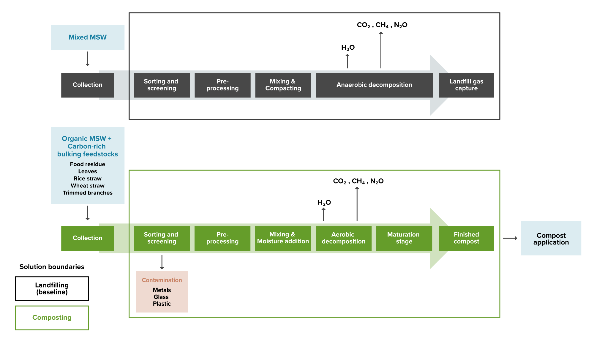
IPCC Task Force on National Greenhouse Gas Inventories. (2019). Refinement to the 2006 IPCC Guidelines for National Greenhouse Gas Inventories (Calvo Buendia, E., Tanabe, K., Kranjc, A., Baasansuren, J., Fukuda, M., Ngarize S., Osako, A., Pyrozhenko, Y., Shermanau, P. and Federici, S., Eds.). Intergovernmental Panel on Climate Change. Link to source: https://www.ipcc-nggip.iges.or.jp/public/2019rf/pdf/0_Overview/19R_V0_00_Cover_Foreword_Preface_Dedication.pdf 

Isbell, F., Craven, D., Connolly, J., Loreau, M., Schmid, B., Beierkuhnlein, C., Bezemer, T. M., Bonin, C., Bruelheide, H., de Luca, E., Ebeling, A., Griffin, J. N., Guo, Q., Hautier, Y., Hector, A., Jentsch, A., Kreyling, J., Lanta, V., Manning, P., … Eisenhauer, N. (2015). Biodiversity increases the resistance of ecosystem productivity to climate extremes. Nature526(7574), 574–577. https://doi.org/10.1038/nature15374

Jackson, R. B., Banner, J. L., Jobbágy, E. G., Pockman, W. T., & Wall, D. H. (2002). Ecosystem carbon loss with woody plant invasion of grasslands. Nature418(6898), 623–626. https://doi.org/10.1038/nature00910

Jones, K. R., Venter, O., Fuller, R. A., Allan, J. R., Maxwell, S. L., Negret, P. J., & Watson, J. E. M. (2018). One-third of global protected land is under intense human pressure. Science360(6390), 788–791. https://doi.org/10.1126/science.aap9565

Kachler, J., Benra, F., Bolliger, R., Isaac, R., Bonn, A., & Felipe-Lucia, M. R. (2023). Can we have it all? The role of grassland conservation in supporting forage production and plant diversity. Landscape Ecology38(12), 4451–4465. https://doi.org/10.1007/s10980-023-01729-4

Kemp, D. R., Guodong, H., Xiangyang, H., Michalk, D. L., Fujiang, H., Jianping, W., & Yingjun, Z. (2013). Innovative grassland management systems for environmental and livelihood benefits. Proceedings of the National Academy of Sciences110(21), 8369–8374. https://doi.org/10.1073/pnas.1208063110

Kim, J. H., Jobbágy, E. G., & Jackson, R. B. (2016). Trade-offs in water and carbon ecosystem services with land-use changes in grasslands. Ecological Applications26(6), 1633–1644. https://doi.org/10.1890/15-0863.1

Knapp, A. K., Chen, A., Griffin-Nolan, R. J., Baur, L. E., Carroll, C. J. W., Gray, J. E., Hoffman, A. M., Li, X., Post, A. K., Slette, I. J., Collins, S. L., Luo, Y., & Smith, M. D. (2020). Resolving the Dust Bowl paradox of grassland responses to extreme drought. Proceedings of the National Academy of Sciences117(36), 22249–22255. https://doi.org/10.1073/pnas.1922030117

Lambin, E. F., Gibbs, H. K., Heilmayr, R., Carlson, K. M., Fleck, L. C., Garrett, R. D., le Polain de Waroux, Y., McDermott, C. L., McLaughlin, D., Newton, P., Nolte, C., Pacheco, P., Rausch, L. L., Streck, C., Thorlakson, T., & Walker, N. F. (2018). The role of supply-chain initiatives in reducing deforestation. Nature Climate Change8(2), 109–116. https://doi.org/10.1038/s41558-017-0061-1

Lefcheck, J. S., Byrnes, J. E. K., Isbell, F., Gamfeldt, L., Griffin, J. N., Eisenhauer, N., Hensel, M. J. S., Hector, A., Cardinale, B. J., & Duffy, J. E. (2015). Biodiversity enhances ecosystem multifunctionality across trophic levels and habitats. Nature Communications6(1), Article 6936. https://doi.org/10.1038/ncomms7936

Levy, S. A., Cammelli, F., Munger, J., Gibbs, H. K., & Garrett, R. D. (2023). Deforestation in the Brazilian Amazon could be halved by scaling up the implementation of zero-deforestation cattle commitments. Global Environmental Change80, Article 102671. https://doi.org/10.1016/j.gloenvcha.2023.102671

Li, G., Fang, C., Watson, J. E. M., Sun, S., Qi, W., Wang, Z., & Liu, J. (2024). Mixed effectiveness of global protected areas in resisting habitat loss. Nature Communications15(1), Article 8389. https://doi.org/10.1038/s41467-024-52693-9

Li, J., Huang, L., Cao, W., Wang, J., Fan, J., Xu, X., & Tian, H. (2023). Benefits, potential and risks of China’s grassland ecosystem conservation and restoration. Science of The Total Environment905, Article 167413. https://doi.org/10.1016/j.scitotenv.2023.167413

Liechti, K., & Biber, J.-P. (2016). Pastoralism in Europe: Characteristics and challenges of highland-lowland transhumance. Revue Scientifique Et Technique (International Office of Epizootics)35(2), 561–575. https://doi.org/10.20506/rst.35.2.2541

Macdonald, K., Diprose, R., Grabs, J., Schleifer, P., Alger, J., Bahruddin, Brandao, J., Cashore, B., Chandra, A., Cisneros, P., Delgado, D., Garrett, R., & Hopkinson, W. (2024). Jurisdictional approaches to sustainable agro-commodity governance: The state of knowledge and future research directions. Earth System Governance22, Article 100227. https://doi.org/10.1016/j.esg.2024.100227

Marin, F. R., Zanon, A. J., Monzon, J. P., Andrade, J. F., Silva, E. H. F. M., Richter, G. L., Antolin, L. A. S., Ribeiro, B. S. M. R., Ribas, G. G., Battisti, R., Heinemann, A. B., & Grassini, P. (2022). Protecting the Amazon forest and reducing global warming via agricultural intensification. Nature Sustainability5, 1018–1026. https://doi.org/10.1038/s41893-022-00968-8

McNicol, I. M., Keane, A., Burgess, N. D., Bowers, S. J., Mitchard, E. T. A., & Ryan, C. M. (2023). Protected areas reduce deforestation and degradation and enhance woody growth across African woodlands. Communications Earth & Environment4(1), Article 392. https://doi.org/10.1038/s43247-023-01053-4

Meng, Z., Dong, J., Ellis, E. C., Metternicht, G., Qin, Y., Song, X.-P., Löfqvist, S., Garrett, R. D., Jia, X., & Xiao, X. (2023). Post-2020 biodiversity framework challenged by cropland expansion in protected areas. Nature Sustainability6(7), 758–768. https://doi.org/10.1038/s41893-023-01093-w

Michalk, D. L., Kemp, D. R., Badgery, W. B., Wu, J., Zhang, Y., & Thomassin, P. J. (2019). Sustainability and future food security—A global perspective for livestock production. Land Degradation & Development30(5), 561–573. https://doi.org/10.1002/ldr.3217

Nabuurs, G.-J., Mrabet, R., Hatab, A. A., Bustamante, M., Clark, H., Havlík, P., House, J. I., Mbow, C., Ninan, K. N., Popp, A., Roe, S., Sohngen, B., & Towprayoon, S. (2022). Agriculture, forestry and other land uses (AFOLU). In P. R. Shukla, J. Skea, R. Slade, A. Al Khourdajie, R. van Diemen, D. McCollum, M. Pathak, S. Some, P. Vyas, R. Fradera, M. Belkacemi, A. Hasija, G. Lisboa, S. Luz, & J. Malley (Eds.), Climate change 2022: Mitigation of climate change. Contribution of working group III to the sixth assessment report of the intergovernmental panel on climate change (pp. 747–860). Cambridge University Press. Link to source: https://doi.org/10.1017/9781009157926.009

Nugent, D. T., Baker-Gabb, D. J., Green, P., Ostendorf, B., Dawlings, F., Clarke, R. H., & Morgan, J. W. (2022). Multi-scale habitat selection by a cryptic, critically endangered grassland bird—The Plains-wanderer (Pedionomus torquatus): Implications for habitat management and conservation. Austral Ecology47(3), 698–712. https://doi.org/10.1111/aec.13157

Olson, D. M., Dinerstein, E., Wikramanayake, E. D., Burgess, N. D., Powell, G. V. N., Underwood, E. C., D’amico, J. A., Itoua, I., Strand, H. E., Morrison, J. C., Loucks, C. J., Allnutt, T. F., Ricketts, T. H., Kura, Y., Lamoreux, J. F., Wettengel, W. W., Hedao, P., & Kassem, K. R. (2001). Terrestrial ecoregions of the world: A new map of life on Earth: A new global map of terrestrial ecoregions provides an innovative tool for conserving biodiversity. BioScience51(11), 933–938. https://doi.org/10.1641/0006-3568(2001)051[0933:TEOTWA]2.0.CO;2

Parente, L., Sloat, L., Mesquita, V., Consoli, D., Stanimirova, R., Hengl, T., Bonannella, C., Teles, N., Wheeler, I., Hunter, M., Ehrmann, S., Ferreira, L., Mattos, A. P., Oliveira, B., Meyer, C., Şahin, M., Witjes, M., Fritz, S., Malek, Z., & Stolle, F. (2024a). Annual 30-m maps of global grassland class and extent (2000–2022) based on spatiotemporal Machine Learning. Scientific Data11(1), Article 1303. https://doi.org/10.1038/s41597-024-04139-6

Parente, L., Sloat, L., Mesquita, V., Consoli, D., Stanimirova, R., Hengl, T., Bonannella, C., Teles, N., Wheeler, I., Hunter, M., Ehrmann, S., Ferreira, L., Mattos, A. P., Oliveira, B., Meyer, C., Şahin, M., Witjes, M., Fritz, S., Malek, Ž., & Stolle, F. (2024b). Global Pasture Watch—Annual grassland class and extent maps at 30-m spatial resolution (2000—2022) (Version v1) [Data set]. Zenodo. https://doi.org/10.5281/zenodo.13890417

Pelser, A., Redelinghuys, N., & Kernan, A.-L. (2015). Protected Areas and ecosystem services—Integrating grassland conservation with human well-being in South Africa. In Biodiversity in Ecosystems—Linking Structure and Function. IntechOpen. https://doi.org/10.5772/59015

Petermann, J. S., & Buzhdygan, O. Y. (2021). Grassland biodiversity. Current Biology31(19), R1195–R1201. https://doi.org/10.1016/j.cub.2021.06.060

Poeplau, C. (2021). Grassland soil organic carbon stocks along management intensity and warming gradients. Grass and Forage Science76(2), 186–195. https://doi.org/10.1111/gfs.12537

Poggio, L., de Sousa, L. M., Batjes, N. H., Heuvelink, G. B. M., Kempen, B., Ribeiro, E., & Rossiter, D. (2021). SoilGrids 2.0: Producing soil information for the globe with quantified spatial uncertainty. SOIL7(1), 217–240. https://doi.org/10.5194/soil-7-217-2021

Ratajczak, Z., Nippert, J. B., & Collins, S. L. (2012). Woody encroachment decreases diversity across North American grasslands and savannas. Ecology93(4), 697–703. https://doi.org/10.1890/11-1199.1

Resare Sahlin, K., Gordon, L. J., Lindborg, R., Piipponen, J., Van Rysselberge, P., Rouet-Leduc, J., & Röös, E. (2024). An exploration of biodiversity limits to grazing ruminant milk and meat production. Nature Sustainability7(9), 1160–1170. https://doi.org/10.1038/s41893-024-01398-4

Saura, S., Bertzky, B., Bastin, L., Battistella, L., Mandrici, A., & Dubois, G. (2019). Global trends in protected area connectivity from 2010 to 2018. Biological Conservation238, Article 108183. https://doi.org/10.1016/j.biocon.2019.07.028

Sloat, L., Balehegn, M., & Johnson, P. (2025, May 2). Grasslands Are Some of Earth’s Most Underrated Ecosystems. World Resources Institute. https://www.wri.org/insights/grassland-benefits

Smith, M. D., Wilkins, K. D., Holdrege, M. C., Wilfahrt, P., Collins, S. L., Knapp, A. K., Sala, O. E., Dukes, J. S., Phillips, R. P., Yahdjian, L., Gherardi, L. A., Ohlert, T., Beier, C., Fraser, L. H., Jentsch, A., Loik, M. E., Maestre, F. T., Power, S. A., Yu, Q., … Zuo, X. (2024). Extreme drought impacts have been underestimated in grasslands and shrublands globally. Proceedings of the National Academy of Sciences121(4), Article e2309881120. https://doi.org/10.1073/pnas.2309881120

Spawn, S. A., Sullivan, C. C., Lark, T. J., & Gibbs, H. K. (2020). Harmonized global maps of above and belowground biomass carbon density in the year 2010. Scientific Data7(1), Article 112. https://doi.org/10.1038/s41597-020-0444-4

Stanley, P. L., Wilson, C., Patterson, E., Machmuller, M. B., & Cotrufo, M. F. (2024). Ruminating on soil carbon: Applying current understanding to inform grazing management. Global Change Biology30(3), Article e17223. https://doi.org/10.1111/gcb.17223

Su, X., Han, W., Liu, G., Zhang, Y., & Lu, H. (2019). Substantial gaps between the protection of biodiversity hotspots in alpine grasslands and the effectiveness of protected areas on the Qinghai-Tibetan Plateau, China. Agriculture, Ecosystems & Environment278, 15–23. https://doi.org/10.1016/j.agee.2019.03.013

Suttie, J. M., Reynolds, S. G., & Batello, C. (Eds.). (2005). Grasslands of the world (Vol. 34). Food and Agriculture Organization of the United Nations. Link to source: https://www.fao.org/4/y8344e/y8344e00.htm 

Sze, J. S., Carrasco, L. R., Childs, D., & Edwards, D. P. (2021). Reduced deforestation and degradation in Indigenous Lands pan-tropically. Nature Sustainability5(2), 123–130. https://doi.org/10.1038/s41893-021-00815-2

United Nations Environment Programme World Conservation Monitoring Centre, & International Union for Conservation of Nature. (2024). Protected planet: The world database on protected areas (WDPA) and world database on other effective area-based conservation measures (WD-OECM) [Data set]. Retrieved November 2024, from https://www.protectedplanet.net

Vijay, V., Fisher, J. R. B., & Armsworth, P. R. (2022). Co-benefits for terrestrial biodiversity and ecosystem services available from contrasting land protection policies in the contiguous United States. Conservation Letters15(5), Article e12907. https://doi.org/10.1111/conl.12907

Villoria, N., Garrett, R., Gollnow, F., & Carlson, K. (2022). Leakage does not fully offset soy supply-chain efforts to reduce deforestation in Brazil. Nature Communications13(1), Article 5476. https://doi.org/10.1038/s41467-022-33213-z

Visconti, P., Butchart, S. H. M., Brooks, T. M., Langhammer, P. F., Marnewick, D., Vergara, S., Yanosky, A., & Watson, J. E. M. (2019). Protected area targets post-2020. Science364(6437), 239–241. https://doi.org/10.1126/science.aav6886

Wade, C. M., Austin, K. G., Cajka, J., Lapidus, D., Everett, K. H., Galperin, D., Maynard, R., & Sobel, A. (2020). What is threatening forests in Protected Areas? A global assessment of deforestation in Protected Areas, 2001–2018. Forests11(5), Article 539. https://doi.org/10.3390/f11050539

Waldron, A., Adams, V., Allan, J., Arnell, A., Asner, G., Atkinson, S., Baccini, A., Baillie, J. E. M., Balmford, A., Beau, J. A., Brander, L., Brondizio, E., Bruner, A., Burgess, N., Burkart, K., Butchart, S., Button, R., Carrasco, R., Cheung, W., … Zhang, Y. P. (2020). Protecting 30% of the planet for nature: Costs, benefits and economic implications [Working paper]. International Institute for Applied Systems Analysis. Link to source: https://pure.iiasa.ac.at/id/eprint/16560/1/Waldron_Report_FINAL_sml.pdf

Ward, M., Saura, S., Williams, B., Ramírez-Delgado, J. P., Arafeh-Dalmau, N., Allan, J. R., Venter, O., Dubois, G., & Watson, J. E. M. (2020). Just ten percent of the global terrestrial protected area network is structurally connected via intact land. Nature Communications11(1), Article 4563. https://doi.org/10.1038/s41467-020-18457-x

Watson, J. E. M., Dudley, N., Segan, D. B., & Hockings, M. (2014). The performance and potential of protected areas. Nature515(7525), 67–73. https://doi.org/10.1038/nature13947

West, T. A. P., Wunder, S., Sills, E. O., Börner, J., Rifai, S. W., Neidermeier, A. N., Frey, G. P., & Kontoleon, A. (2023). Action needed to make carbon offsets from forest conservation work for climate change mitigation. Science381(6660), 873–877. https://doi.org/10.1126/science.ade3535

Williams, M., Reay, D., & Smith, P. (2023). Avoiding emissions versus creating sinks—Effectiveness and attractiveness to climate finance. Global Change Biology29(8), 2046–2049. https://doi.org/10.1111/gcb.16598

Wolf, C., Levi, T., Ripple, W. J., Zárrate-Charry, D. A., & Betts, M. G. (2021). A forest loss report card for the world’s protected areas. Nature Ecology & Evolution5(4), 520–529. https://doi.org/10.1038/s41559-021-01389-0

Yao, J., Liu, H., Huang, J., Gao, Z., Wang, G., Li, D., Yu, H., & Chen, X. (2020). Accelerated dryland expansion regulates future variability in dryland gross primary production. Nature Communications11(1), Article 1665. https://doi.org/10.1038/s41467-020-15515-2

Yu, Q., Xu, C., Wu, H., Ke, Y., Zuo, X., Luo, W., Ren, H., Gu, Q., Wang, H., Ma, W., Knapp, A. K., Collins, S. L., Rudgers, J. A., Luo, Y., Hautier, Y., Wang, C., Wang, Z., Jiang, Y., Han, G., … Han, X. (2025). Contrasting drought sensitivity of Eurasian and North American grasslands. Nature639(8053), 114–118. https://doi.org/10.1038/s41586-024-08478-7

Zhu, K., Chiariello, N. R., Tobeck, T., Fukami, T., & Field, C. B. (2016). Nonlinear, interacting responses to climate limit grassland production under global change. Proceedings of the National Academy of Sciences113(38), 10589–10594. https://doi.org/10.1073/pnas.1606734113

Zhu, K., Song, Y., Lesage, J. C., Luong, J. C., Bartolome, J. W., Chiariello, N. R., Dudney, J., Field, C. B., Hallett, L. M., Hammond, M., Harrison, S. P., Hayes, G. F., Hobbs, R. J., Holl, K. D., Hopkinson, P., Larios, L., Loik, M. E., & Prugh, L. R. (2024). Rapid shifts in grassland communities driven by climate change. Nature Ecology & Evolution8(12), 2252–2264. https://doi.org/10.1038/s41559-024-02552-z

Credits

Lead Fellow

  • Avery Driscoll

Contributors

  • Ruthie Burrows, Ph.D.

  • James Gerber, Ph.D.

  • Daniel Jasper

  • Alex Sweeney

Internal Reviewers

  • Aiyana Bodi

  • Hannah Henkin

  • Ted Otte

  • Christina Richardson, Ph.D.

  • Christina Swanson, Ph.D.

  • Paul C. West, Ph.D.

Effectiveness

We estimated that protecting 1 ha of grasslands avoids 0.06–0.90 t CO₂‑eq/yr, with emissions reductions tending to be higher in boreal and temperate regions than tropical and subtropical regions (100-yr GWP; Table 1a–d; Appendix).

We estimated effectiveness as the avoided emissions attributable to the reduction in grassland conversion conferred by protection (Equation 1; Appendix), assuming that converted grasslands are used as croplands due to data constraints. Although some grasslands are converted to intensively managed pastures or urban development, we assumed that the total land area converted to infrastructure is relatively small and emissions associated with conversion to planted pastures are comparable to those from conversion to cropland.

We aggregated estimates of avoided grassland conversion attributable to PAs from Li et al. (2024) to the biome level (Grassland lossavoided), then multiplied the result by the total emissions over 30 years from 1 ha of grassland converted to cropland. These emissions include the change in biomass and soil carbon on conversion to cropland (Carbonemissions), 30 years of lost carbon sequestration potential (Carbonuptake), and nitrous oxide emissions associated with soil carbon loss, which is a small component of total emissions (see Appendix for details; Chang et al. 2021; Huang et al., 2024; Intergovernmental Panel on Climate Change 2019; Poggio et al., 2021; Spawn et al., 2020).

left_text_column_width

Equation 1.

\[Effectiveness=(Grassland\text{ }loss_{avoided} \times (Carbon_{emissions} + Carbon_{uptake})

The effectiveness of grassland protection as defined here reflects only a small percentage of the carbon stored in grassland because we accounted for the likelihood that the grassland would be converted without protection. Grassland protection is particularly impactful for areas at high risk of conversion.

left_text_column_width

Table 1a–d. Effectiveness of grassland protection at avoiding emissions and sequestering carbon. Regional differences in values are driven by variation in carbon stocks, baseline rates of grassland conversion, and the effectiveness of PAs at reducing conversion.

Unit: t CO₂‑eq (100-yr basis)/ha/yr

Estimate 0.90

Unit: t CO₂‑eq (100-yr basis)/ha/yr

Estimate 0.54

Unit: t CO₂‑eq (100-yr basis)/ha/yr

Estimate 0.13

Unit: t CO₂‑eq (100-yr basis)/ha/yr

Estimate 0.06
Left Text Column Width
Cost

The costs of grassland protection include up-front costs of land acquisition and ongoing costs of management and enforcement. The market price of land reflects the opportunity cost of not using the land for other purposes, such as agriculture or urban development. Data related to the costs of grassland protection are very limited. 

We estimated that grassland protection provides a net cost savings of approximately US$0.53/ha/yr, or US$1.58/t CO₂‑eq avoided (Table 2). This estimate reflects global averages rather than regionally specific values, and some data are not specific to grasslands. Costs and revenues are highly variable across regions, depending on the costs of land and enforcement and the potential for tourism. 

Dienerstein et al. (2024) estimated the initial cost of establishing a PA for 60 high-biodiversity ecoregions. Amongst the 20 regions that contain grasslands, the median acquisition cost was US$897/ha, which we amortized over 30 years. Costs of PA maintenance were estimated at US$9–17/ha/yr (Bruner et al., 2004; Waldron et al., 2020), though these estimates were not specific to grasslands. Additionally, these estimates reflect the costs of effective enforcement and management, but many existing PAs lack adequate funds for effective enforcement (Adams et al., 2019; Barnes et al., 2018; Burner et al., 2004). 

Protecting grasslands can generate revenue through increased tourism. Waldron et al. (2020) estimated that, across all ecosystems, tourism revenues directly attributable to PA establishment were US$43 ha/yr, not including downstream revenues from industries that benefit from increased tourism. Inclusion of a tourism multiplier would substantially increase the estimated economic benefits of grassland protection.

left_text_column_width

Table 2. Cost per unit of climate impact for grassland protection. Negative value indicates cost savings.

Unit: 2023 US$/t CO₂‑eq , 100-yr basis

median -1.58
Left Text Column Width
Learning Curve

A learning curve is defined here as falling costs with increased adoption. The costs of grassland protection do not fall with increasing adoption, so there is no learning curve for this solution.

left_text_column_width
Speed of Action

The term speed of action refers to how quickly a climate solution physically affects the atmosphere after it is deployed. This is separate from the speed of deployment, which is the pace at which solutions are adopted.

At Project Drawdown, we define the speed of action for each climate solution as emergency brake, gradual, or delayed.

Protect Grasslands is an EMERGENCY BRAKE climate solution. It reduces pulses of emissions from the conversion of grasslands, offering the potential to deliver a more rapid impact than gradual and delayed solutions. Because emergency brake solutions can deliver their climate benefits quickly, they can help accelerate our efforts to address dangerous levels of climate change. For this reason, they are a high priority.

left_text_column_width
Caveats

Permanence, or the durability of stored carbon, is a caveat for emissions avoidance through grassland protection that is not addressed in this analysis. Protected grasslands could be converted to agricultural uses or other development if legal protections are reversed or inadequately enforced, resulting in the loss of stored carbon. Many PAs allow for some human uses, and PA management that is not tailored to grazing needs, fire dependency, or woody plant encroachment can reduce carbon stocks within PAs (Barger et al., 2011; Chang et al., 2021; Conant et al, 2017; Jackson et al., 2002; Kemp et al., 2013; Popleau et al., 2011). Climate change is also causing widespread degradation of grasslands, including reductions in vegetation productivity that may reduce carbon storage over the long term even in the absence of additional disturbance (Chang et al., 2021; Gang et al., 2014; Li et al., 2023; Zhu et al., 2016). Climate change and aridification may also cause expansion of grassland extent (Berg & McColl, 2021; Feng & Fu, 2014; Huang et al., 2016), with mixed but overall negative impacts on terrestrial carbon uptake (Yao et al., 2020).

Additionality, or the degree to which emissions reductions are above and beyond a baseline, is another important caveat for emissions avoidance through ecosystem protection (Ahlering et al., 2016; Williams et al., 2023). In this analysis, additionality was addressed by using baseline rates of grassland conversion in calculating effectiveness. Evaluating additionality is challenging and remains an active area of research.

left_text_column_width
Current Adoption

A total of 555 Mha of grasslands (excluding grasslands on peat soils, grasslands that are also coastal wetlands, and grasslands created through deforestation) are currently located within PAs, and an additional 832 Mha are located on IPLs not classified as PAs (Table 3e). That means that ~48% of grasslands are under some form of protection globally, with 6% in strict PAs, 13% in non-strict PAs, and 29% on IPLs that are not also PAs. As of 2023, tropical regions had the largest extent of protected grasslands (583 Mha), followed by boreal regions (339 Mha), and subtropical regions (293 Mha). In temperate regions, only 24% of grasslands (172 Mha) were under any form of protection (Table 3a–d).

left_text_column_width

Table 3a–e. Grassland under protection by biome (circa 2023). Estimates are provided for three different forms of protection: “strict” protection, including IUCN classes I and II; “non-strict” protection, including all other IUCN categories; and IPLs outside of PAs. Regional values may not sum to global totals due to rounding.

Unit: ha protected

Strict PAs 52,564,000
Non-strict PAs 82,447,000
IPLs 203,579,000

Unit: ha protected

Strict PAs 30,242,000
Non-strict PAs 51,033,000
IPLs 90,973,000

Unit: ha protected

Strict PAs 31,949,000
Non-strict PAs 83,745,000
IPLs 177,301,000

Unit: ha protected

Strict PAs 56,233,000
Non-strict PAs 166,356,000
IPLs 359,997,000

Unit: ha protected

Strict PAs 170,988,000
Non-strict PAs 383,581,000
IPLs 831,850,000
Left Text Column Width
Adoption Trend

We calculated the annual rate of new grassland protection based on the year of PA establishment for areas established in 2000–2020. The median annual increase in grassland protection was 8.1 Mha (mean 11.4 Mha; Table 4e). This represents a roughly 1.5%/yr increase in grasslands within PAs, or protection of an additional 0.3%/yr of total global grasslands. 

Grassland protection has proceeded more quickly in tropical regions (median increase of 4.0 Mha/yr) than in other climate zones (median increases of 1.2–1.6 Mha/yr) (Table 4a–d). Although the global rate of grassland protection fluctuates from year to year, the median rate has remained stable in recent decades at 10.2 Mha/yr from 2000–2009 and 10.4 Mha/yr from 2010–2020. 

left_text_column_width

Table 4a–e. Adoption trend for grassland protection in PAs of any IUCN class (2000–2020). The 25th and 75th percentiles reflect only interannual variance (ha grassland protected/yr). IPLs are not included in this analysis due to a lack of data.

Unit: ha grassland protected/yr

25th percentile 659,000
median (50th percentile) 1,338,000
mean 2,152,000
75th percentile 3,007,000

Unit: ha grassland protected/yr

25th percentile 692,000
median (50th percentile) 1,178,000
mean 1,728,000
75th percentile 1,715,000

Unit: ha grassland protected/yr

25th percentile 940,000
median (50th percentile) 1,580,000
mean 2,791,000
75th percentile 3,226,000

Unit: ha grassland protected/yr

25th percentile 2,628,000
median (50th percentile) 4,044,000
mean 4,711,000
75th percentile 5,774,000

Unit: ha grassland protected/yr

25th percentile 4,919,000
median (50th percentile) 8,140,000
mean 11,382,000
75th percentile 13,722,000
Left Text Column Width
Adoption Ceiling

Including grasslands that are currently protected, we estimated that there are approximately 2,891 Mha of natural grasslands that are not counted in a different solution (Table 5e). This ceiling includes 1,505 Mha that are not currently under any form of protection. This includes 533 Mha of eligible grasslands in boreal regions, 723 Mha in temperate regions, 626 Mha in the subtropics, and 1,008 Mha in the tropics (Table 5a–d). 

To develop these estimates, we relied on the global grassland map from Parente et al. (2024), excluded areas that were included in the Protect ForestsProtect Peatlands, and Protect Coastal Wetlands solutions, and excluded areas that were historically forested according to the Terrestrial Ecoregions of The World dataset (Olson et al., 2001; Appendix). While it is not socially, politically, or economically realistic that all remaining grasslands could be protected, these values represent the technical upper limit to adoption of this solution.

left_text_column_width

Table 5a–e. Adoption ceiling: upper limit for adoption of legal protection of grasslands by biome. Values may not sum to global totals due to rounding. 

Unit: ha protected

Estimate 533,033,000

Unit: ha protected

Estimate 723,429,000

Unit: ha protected

Estimate 626,474,000

Unit: ha protected

Estimate 1,008,375,000

Unit: ha protected

Estimate 2,891,311,000
Left Text Column Width
Achievable Adoption

We assigned a low achievable level of a minimum of 50% of grasslands in each climate zone (Table 6a–e). For boreal and tropical regions, in which 64% and 58%, respectively, of grasslands are already protected, we assume no change in PA (Table 6a, d). For temperate areas, the low achievable target reflects an increase of 189 Mha, or more than a doubling of the current PA extent (Table 6b). In subtropical zones, this target reflects an additional 20 Mha under protection (Table 6c). We assigned a high achievable level of 70% of grasslands in each climate zone, reflecting an additional 637 Mha of protected grasslands globally, or a 46% increase in the current PA extent (Table 6a–e).

left_text_column_width

Table 6a–e. Range of achievable adoption of grassland protection by biome.

Unit: ha protected

Current Adoption 338,590,000
Achievable – Low 338,590,000
Achievable – High 373,123,000
Adoption ceiling 533,033,000

Unit: ha protected

Current Adoption 172,248,000
Achievable – Low 361,715,000
Achievable – High 506,400,000
Adoption ceiling 723,429,000

Unit: ha protected

Current Adoption 292,995,000
Achievable – Low 313,237,000
Achievable – High 438,532,000
Adoption ceiling 626,474,000

Unit: ha protected

Current Adoption 582,586,000
Achievable – Low 582,586,000
Achievable – High 705,863,000
Adoption ceiling 1,008,375,000

Unit: ha protected

Current Adoption 1,386,419,000
Achievable – Low 1,596,128,000
Achievable – High 2,023,918,000
Adoption ceiling 2,891,311,000
Left Text Column Width

We estimated that PAs currently reduce GHG emissions from grassland conversion by 0.468 Gt CO₂‑eq/yr (Table 7a–e). Achievable levels of grassland protection have the potential to reduce emissions 0.572–0.704 Gt CO₂‑eq/yr, with a technical upper bound of 1.006 Gt CO₂‑eq/yr (Table 7a–e). This indicates that further emissions reductions of 0.105–0.237 Gt CO₂‑eq/yr are achievable. For these benefits to be realized, grazing, fire, and woody plant management must be responsive to local grassland needs and compatible with the maintenance of carbon stocks. The solutions Improve Livestock Grazing and Deploy Silvopasture address the climate impacts of some aspects of grassland management.

Few other sources explicitly quantify the climate impacts of grassland protection, but the available data are roughly aligned with our estimates of additional mitigation potential. The Intergovernmental Panel on Climate Change estimated that avoided conversion of grasslands to croplands could reduce emissions by 0.03–0.7 Gt CO₂‑eq/yr (Nabuurs et al., 2022). Griscom et al. (2017) estimated that avoided grassland conversion could save 0.12 Gt CO₂‑eq/yr emissions from soil carbon only (not counting loss of vegetation, sequestration potential, or nitrous oxide), though their analysis did not account for current protection and relied on older estimates of grassland conversion. 

left_text_column_width

Table 7a–e. Climate impact at different levels of adoption.

Unit: GtCO₂‑eq/yr, 100-year basis

Current Adoption 0.305
Achievable – Low 0.305
Achievable – High 0.336
Adoption Ceiling 0.481

Unit: GtCO₂‑eq/yr, 100-year basis

Current Adoption 0.093
Achievable – Low 0.195
Achievable – High 0.273
Adoption Ceiling 0.390

Unit: GtCO₂‑eq/yr, 100-year basis

Current Adoption 0.037
Achievable – Low 0.039
Achievable – High 0.055
Adoption Ceiling 0.078

Unit: GtCO₂‑eq/yr, 100-year basis

Current Adoption 0.033
Achievable – Low 0.033
Achievable – High 0.040
Adoption Ceiling 0.057

Unit: GtCO₂‑eq/yr, 100-year basis

Current Adoption 0.468
Achievable – Low 0.572
Achievable – High 0.704
Adoption Ceiling 1.006
Left Text Column Width
Additional Benefits

Floods

Grassland plants often have deep root systems, leading to high soil carbon stocks (Sloat et al., 2025). These roots can absorb water and reduce discharge into surrounding water bodies during periods of excessive rain (GRaSS, 2024).

Droughts

Different grassland plant species respond differently to drought. Differences in precipitation seasonality due to drought may allow some grass species to dominate over others (Knapp et al., 2020). Evidence suggests that higher species diversity can enhance grassland resilience to drought (Smith et al., 2024; Yu et al., 2025).  Additionally, the deep root systems of grassland plants contribute to the drought resilience of these ecosystems (Sloat et al., 2025). More resilient, biodiverse grasslands are associated with greater ecosystem stability and productivity, and can maintain ecosystem services during periods of extreme weather, such as drought (Isbell et al, 2015; Lefcheck et al., 2015).

Income and Work

Grasslands are an important source of income for surrounding communities through tourism and other ecosystem services (Bengtsson et al., 2019). Protecting grasslands sustains the long-term health of the ecosystem, which is especially important for subsistence livelihoods that depend on intact landscapes for incomes (Pelser, 2015). Sources of income that are directly generated from grasslands include: meat, milk, wool, and leather and thatching materials to make brooms, hats, and baskets (GRaSS, 2024; Pelser, 2015). People living near grasslands often rely on grazing livestock for food and income (GRaSS, 2024, Kemp 2013, Su et al., 2019). Grasslands in China support the livelihoods of about 16 million people, many of whom live in poverty (Kemp et al., 2013). The Qinghai-Tibetan Plateau is especially important for grazing livestock (Su et al., 2019). Evidence has shown that declines in grassland productivity are also linked to declines in income (Kemp et al., 2013).

Food Security

Grasslands can contribute to food security by providing food for livestock and supporting pollinators for nearby agriculture (Sloat et al., 2025). Grassland-based grazing systems are important sources of food for populations in low and middle-income countries, particularly in Oceania, Latin America, the Caribbean, the Middle East, North Africa, and sub-Saharan Africa (Resare Sahlin et al., 2023). Grasslands can support the food security of smallholder farmers and pastoralists in these regions by providing meat and milk (GRaSS, 2024; Michalk, 2018). 

Equality

Grasslands are central to many cultures, and grassland protection can support shared cultural and spiritual values for many populations. They can be sources of identity for people living in or near grassland ecosystems who have strong connections with the land (Bengtsson et al., 2019, GRaSS, 2024). For example, in Mongolia grasslands sustain horses, which are central to the cultural identities and livelihoods of communities, particularly nomadic populations (Kemp et al., 2014). Grasslands can also be an important source of shared identity for pastoralists who move herds to graze based on seasonal cycles during the year (Liechti & Biber, 2016).

Nature Protection

Many grasslands are biodiversity hot spots (Petermann & Buzhdygan, 2021; Su et al., 2019). Numerous plant and animal species are endemic to grasslands, meaning they have limited habitat ranges and can easily become endangered with habitat degradation (Sloat et al., 2025). In Germany, grasslands in PAs were found to have higher plant diversity than in non-PAs (Kachler et al., 2023). Grasslands are important habitats for bird species that rely on them for breeding grounds (GRaSS, 2024; Nugent et al., 2022).

Land Resources

The unique, deep root structures of some grassland plants can improve soil stability and reduce soil erosion (Bengtsson et al., 2019; GRaSS, 2024; Kemp et al., 2013).

Water Resources

Grasslands can regulate water flows and water storage. The root systems can help rainwater reach deep underground, recharging groundwater stores (Bengtsson et al., 2019; GRaSS, 2024).

left_text_column_width
Risks

Relying on grassland protection as an emissions reduction strategy can be undermined if ecosystem conversion that is not allowed inside a PA simply takes place outside of it instead (Aherling et al., 2016; Asamoah et al., 2021). If such leakage leads to conversion of ecosystems that have higher carbon stocks, such as forests, peatlands, or coastal wetlands, total emissions may increase. Combining grassland protection with policies to reduce incentives for ecosystem conversion can help avoid leakage.

left_text_column_width
Interactions with Other Solutions

Reinforcing

PAs often include multiple ecosystems. Grassland protection will likely lead to protection of other ecosystems within the same areas, and the health of nearby ecosystems is improved by the services provided by intact grasslands. 

left_text_column_width

These solutions reduce pressure to convert grasslands to agricultural use, easing the expansion of PAs.

left_text_column_width

Restored grasslands need protection to reduce the risk of future disturbance, and the health of protected grasslands can be improved through the restoration of adjacent degraded grasslands.

left_text_column_width

Grazing by large herbivores is critical for the health of many grasslands, and healthy grasslands are needed to support restoration of large herbivores.

left_text_column_width

Competing

Additional crop deployment can increase demand for agricultural land, reducing the grassland area available for protection. 

left_text_column_width

Grassland protection may reduce land availability for renewable energy infrastructure.

left_text_column_width
Dashboard

Solution Basics

ha of grassland or savanna protected

t CO₂-eq (100-yr)/unit/yr
0.9
units
Current 3.386×10⁸ 03.386×10⁸3.731×10⁸
Achievable (Low to High)

Climate Impact

Gt CO₂-eq (100-yr)/yr
Current 0.305 0.3050.336
US$ per t CO₂-eq
-2
Emergency Brake

CO₂,  N₂O

Solution Basics

ha of grassland or savanna protected

t CO₂-eq (100-yr)/unit/yr
0.54
units
Current 1.722×10⁸ 03.617×10⁸5.064×10⁸
Achievable (Low to High)

Climate Impact

Gt CO₂-eq (100-yr)/yr
Current 0.093 0.1950.273
US$ per t CO₂-eq
-2
Emergency Brake

CO₂,  N₂O

Solution Basics

ha of grassland or savanna protected

t CO₂-eq (100-yr)/unit/yr
0.13
units
Current 2.93×10⁸ 03.132×10⁸4.385×10⁸
Achievable (Low to High)

Climate Impact

Gt CO₂-eq (100-yr)/yr
Current 0.037 0.0390.055
US$ per t CO₂-eq
-2
Emergency Brake

CO₂,  N₂O

Solution Basics

ha of grassland or savanna protected

t CO₂-eq (100-yr)/unit/yr
0.06
units
Current 5.826×10⁸ 05.826×10⁸7.059×10⁸
Achievable (Low to High)

Climate Impact

Gt CO₂-eq (100-yr)/yr
Current 0.033 0.0330.04
US$ per t CO₂-eq
-2
Emergency Brake

CO₂,  N₂O

Trade-offs

Establishment of PAs may limit local access to grasslands for grazing or other forms of income generation, although effective management plans should account for the grazing needs of the protected grassland. Second, allocation of budgetary resources to PA establishment may divert resources from maintenance and enforcement of existing PAs. Finally, protection of grasslands may reduce land availability for renewable energy infrastructure, such as solar and wind power.

left_text_column_width
Action Word
Protect
Solution Title
Grasslands & Savannas
Classification
Highly Recommended
Lawmakers and Policymakers
  • Set scalable targets (across both biogeographic and administrative levels) for grassland protections, including outcomes-based reporting, indicators for the rate of progress, goals for inclusivity, and measurements for enforcement efficacy; incorporate these targets into national climate plans and multilateral agreements.
  • Ensure public procurement uses products and supply chains that do not disrupt PAs and grasslands; ensure public development projects do not disturb PAs and grasslands.
  • Grant Indigenous communities full property rights and autonomy and support them in monitoring, managing, and enforcing PAs; adhere to principles of free, prior, and informed consent when engaging with Indigenous communities and lands.
  • Manage fire, biodiversity, and grazing in protected grasslands in accordance with ecological needs, learning from and working with Indigenous communities.
  • Ensure PAs don’t displace, violate rights, or reduce access to vital resources for local and Indigenous communities.
  • Expand regulatory, legal, and technical support for privately protected grasslands.
  • When expanding PAs, acquire relevant adjacent properties first, if possible, to increase connectivity and reduce costs; grant restored grasslands protected status.
  • Invest in PA infrastructure, monitoring, management, and enforcement mechanisms.
  • Ban or restrict overgrazing and extractive harvesting while allowing for sustainable use of PAs from Indigenous and local communities; compensate herders for lost grazing lands, if necessary.
  • Ensure PAs are adequately financed and, if applicable, provide financing for low- and middle-income countries and communities for grassland protections.
  • Ensure incentives and/or compensation for reducing livestock or protecting grasslands are evenly distributed with particular attention to low- and middle-income farmers and communities.
  • Use financial incentives such as subsidies, tax breaks, payments for ecosystem services (PES), and debt-for-nature swaps to protect grasslands from development.
  • Remove harmful subsidies for agricultural, grazing, mining, and other resource extraction.
  • Use co-management, community-governed, land-trust, and/or privately protected models to expand PAs, increase connectivity, and engage communities; ensure a participatory approach to designating and managing PAs.
  • Use real-time monitoring, ground-level sensors, and satellite data to enforce protections, ensuring adequate baseline data are gathered if possible.
  • Ensure budgets adequately split financing between expanding PAs and managing PAs; prioritize quality management of existing PAs before expanding new designations except in cases where nonprotected land conversion presents the most serious risks to people, the climate, or biodiversity.
  • Conduct proactive land-use planning to avoid roads and other development projects that may interfere with PAs or incentivize development.
  • Create processes for legal grievances, dispute resolution, and restitution.
  • Create programs that educate the public on PA regulations, the benefits of the regulations, and how to use grassland resources sustainably.
  • Join, support, or create certification and independent audit schemes to monitor effectiveness and identify necessary improvements in management.
Practitioners
  • Set scalable targets (across both biogeographic and administrative levels) for grassland protection, including outcomes-based reporting, indicators for the rate of progress, goals for inclusivity, and measurements for enforcement efficacy; advocate to incorporate these targets into national climate plans and multilateral agreements.
  • Improve monitoring and evaluation standards for grassland ecologies and the impacts from animal agriculture.
  • Ensure incentives and/or compensation for reducing livestock or protecting grasslands are evenly distributed with particular attention to low- and middle-income farmers and communities.
  • Ensure PAs are adequately financed and, if applicable, provide financing for low- and middle-income countries and communities for grassland protections.
  • When expanding PAs, acquire relevant adjacent properties first, if possible, to increase connectivity and reduce costs.
  • Use financial incentives such as subsidies, tax breaks, PES, and debt-for-nature swaps to protect grasslands from development.
  • Empower local communities to manage grasslands and ensure a participatory approach to designating and managing PAs.
  • Use co-management, community-governed, land-trust, and/or privately-protected models to expand PAs, increase connectivity, and engage communities.
  • Ban or restrict overgrazing and extractive harvesting while allowing sustainable use of PAs by Indigenous and local communities; compensate herders for lost grazing lands if necessary.
  • Use real-time monitoring, ground-level sensors, and satellite data to enforce protections, ensuring adequate baseline data are gathered if possible.
  • Ensure budgets adequately split financing between expanding PAs and managing PAs; prioritize quality management of existing PAs before expanding new designations - except in cases where non-protected land conversion presents the most serious risk to people, the climate, or biodiversity.
  • Create education programs that educate the public on PA regulations, the benefits of the regulations, and how to use grassland resources sustainably.
  • Join, support, or create certification and independent audit schemes to monitor effectiveness and identify necessary improvements in management.
Business Leaders
  • Ensure operations, development, and supply chains are not degrading grasslands or interfering with PA management.
  • Integrate grassland protection into net-zero strategies, if relevant.
  • Commit and adhere to minimizing irrecoverable carbon loss through development projects, supply-chain management, and general operations.
  • Help revise existing or create new high-integrity carbon markets, institutions, rules, and norms to cultivate the demand for high-quality carbon credits.
  • Only purchase carbon credits from high-integrity, verifiable carbon markets, and do not use them as replacements for decarbonizing operations or claim them as “offsets.”
  • Consider donating to established grassland protection funds in place of carbon credits.
  • Take advantage of financial incentives such as subsidies, tax breaks, and PES to grasslands from development.
  • Amplify the voices of local communities and civil society to promote robust media coverage.
  • Invest in and support Indigenous and local communities' capacity for management, legal protection, and public relations.
  • Leverage political influence to advocate for stronger grassland protection policies at national and international levels.
  • Conduct proactive land use planning to avoid roads and other development projects that may interfere with PAs.
  • Join, support, or create certification and independent audit schemes to monitor effectiveness and identify necessary improvements in management.

Further information:

Nonprofit Leaders
  • Advocate for enhanced enforcement of existing PAs and IPLs, expansion of new PAs and IPLs, and for more public investments.
  • Advocate for scalable targets (across both biogeographic and administrative levels) for grassland protections, including outcomes-based reporting, indicators for the rate of progress, goals for inclusivity, and measurements for enforcement efficacy; advocate for these goals to be incorporated into national climate plans and multilateral agreements.
  • Help manage and monitor protected grasslands using real-time monitoring, ground-based sensors, and satellite data.
  • Provide financial support for monitoring and enforcement of PAs and IPLs.
  • Help conduct proactive land-use planning to avoid infrastructure or development projects that may interfere with protected grasslands or incentivize destruction.
  • Advocate for creating legal grievance processes, dispute resolution mechanisms, and restitution procedures for violations or disagreements over PAs or IPLs.
  • Help revise existing or create new high-integrity carbon markets, institutions, rules, and norms to cultivate the demand for high-quality carbon credits.
  • Amplify the voices of local communities and civil society to promote robust media coverage.
  • Invest in and support the capacity of Indigenous and local communities for management, legal protection, and public relations.
  • Use or advocate for financial incentives such as subsidies, tax breaks, and PES to protect grasslands from development.
  • Improve monitoring and evaluation standards for grassland ecologies and the impacts from animal agriculture.
  • Help classify and map grasslands, carbon stocks, and biodiversity data and create local, national, and international standards for classification.
  • Work with insurance companies to reduce insurance premiums for properties that protect or maintain grasslands.
  • Create and manage a global database of protected grasslands, grassland loss, restoration, and management initiatives.
  • Join, support, or create certification and independent audit schemes to monitor effectiveness and identify necessary improvements in management.
  • Create programs that educate the public on PA regulations, the benefits of the regulations, and how to use grassland resources sustainably.

Further information:

Investors
  • Ensure investment portfolios do not degrade grasslands or interfere with PAs or IPLs, using data, information, and the latest technology to inform investments.
  • Consider any project that releases irrecoverable carbon loss through the destruction of ecosystems like grasslands to be high risk, avoid investments in these projects as much as possible, and divest from any companies violating this principle.
  • Invest in grassland protection, monitoring, management, and enforcement mechanisms.
  • Use financial mechanisms such as credible biodiversity offsets, payments for ecosystem services, voluntary high-integrity carbon markets, and debt-for-nature swaps to fund grassland protection.
  • Invest in and support the capacity of Indigenous and local communities for management, legal protection, and public relations.
  • Share with other investors and nongovernmental organizations data, information, and investment frameworks that successfully avoid investments that drive grassland destruction.
  • Provide favorable loans to Indigenous communities and entrepreneurs and businesses protecting grasslands.
  • Join, support, or create certification and independent audit schemes to monitor effectiveness and identify necessary improvements in management.

Further information:

Philanthropists and International Aid Agencies
  • Advocate for enhanced enforcement of existing PAs and IPLs, expansion of new PAs and IPLs, and more public investments.
  • Advocate for scalable targets (across both biogeographic and administrative levels) for grassland protections, including outcomes-based reporting, indicators for the rate of progress, goals for inclusivity, and measurements for enforcement efficacy; advocate for these goals to be incorporated into national climate plans and multilateral agreements.
  • Use or advocate for financial incentives such as subsidies, tax breaks, and PES to protect grasslands from development.
  • Help manage and monitor protected grassland, using real-time monitoring and satellite data.
  • Provide technical assistance to low- and middle-income countries and communities for grasslands protection.
  • Provide financial assistance to low- and middle-income countries and communities for grasslands protection.
  • Provide financial support to organizations and institutions developing and deploying monitoring technology and conducting grassland research.
  • Help conduct proactive land-use planning to avoid infrastructure or development projects that may interfere with protected grasslands or incentivize destruction.
  • Help revise existing or create new high-integrity carbon markets, institutions, rules, and norms to cultivate the demand for high-quality carbon credits.
  • Amplify the voices of local communities and civil society to promote robust media coverage.
  • Invest in and support Indigenous and local communities' capacity for management, legal protection, and public relations.
  • Advocate for creating legal grievance processes, dispute resolution mechanisms, and restitution procedures for violations or disagreements over PAs or IPLs.
  • Help classify and map grasslands, carbon stocks, and biodiversity data and create local, national, and international standards for classification.
  • Work with insurance companies to reduce insurance premiums for properties that protect or maintain grasslands.
  • Create and manage a global database of protected grasslands, grassland loss, restoration, and management initiatives.
  • Join, support, or create certification and independent audit schemes to monitor effectiveness and identify necessary improvements in management.
  • Create education programs that educate the public on PA regulations, the benefits of the regulations, and how to use grassland resources sustainably.

Further information:

Thought Leaders
  • Help change the narrative around grasslands by highlighting their value and benefits such as supporting human life, biodiversity, ecosystem resilience, and climate regulation.
  • Advocate for enhanced enforcement of existing PAs and IPLs, expansion of new PAs and IPLs, and public investments.
  • Advocate for scalable targets (across both biogeographic and administrative levels) for grassland protections, including outcomes-based reporting, indicators for the rate of progress, goals for inclusivity, and measurements for enforcement efficacy; advocate for these to be incorporated into national climate plans and multilateral agreements.
  • Advocate for or use financial incentives such as subsidies, tax breaks, PES, and debt-for-nature swaps to protect grasslands from development.
  • Help manage and monitor protected grasslands using real-time monitoring and satellite data.
  • Help conduct proactive land-use planning to avoid infrastructure or development projects that may interfere with protected grasslands or incentivize conversion.
  • Advocate for creating legal grievance processes, dispute resolution mechanisms, and restitution procedures for violations or disagreements over PAs or IPLs.
  • Help improve monitoring and evaluation standards for grassland ecologies and impacts from animal agriculture.
  • Help revise existing or create new high-integrity carbon and biodiversity markets, institutions, rules, and norms to cultivate the demand for high-quality carbon credits.
  • Amplify the voices of local communities and civil society to promote robust media coverage.
  • Support Indigenous and local communities' capacity for legal protection, management, and public relations.
  • Help classify and map grasslands, carbon stocks, and biodiversity data and create local, national, and international standards for classification.
  • Create and manage a global database of protected grasslands, grassland loss, restoration, and management initiatives.
  • Join, support, or create certification and independent audit schemes to monitor effectiveness and identify necessary improvements in management.
  • Create programs that educate the public on PA regulations, the benefits of the regulations, and how to use grassland resources sustainably.

Further information:

Technologists and Researchers
  • Develop standardized indicators of grassland degradation.
  • Research the ecological interactions of grasslands with other ecosystems; share data widely and include recommendations for coordinated action.
  • Assess and publish costs of PA designation, management, and evaluation.
  • Conduct comparative analysis on different types of governance models for PAs to determine impacts on climate, biodiversity, and human well-being.
  • Examine the relationship between geography and governance structures of private PAs, looking for spatial patterns and roles of various stakeholders such NGOs, businesses, and private landowners.
  • Study behavioral change mechanisms that can increase effectiveness and enforcement of PAs.
  • Improve monitoring methods using field measurements, models, satellite imagery, and GIS tools.
  • Create or improve on existing software tools that allow for dynamic planning and management of PAs by monitoring impacts on local communities, the climate, and biodiversity.
  • Create local research sites to support PAs and provide technical assistance.
  • Create tools for local communities to monitor grasslands, such as mobile apps, e-learning platforms, and mapping tools.
  • Develop supply chain tracking software for investors and businesses seeking to create sustainable portfolios and products.

Further information:

Communities, Households, and Individuals
  • Avoid developing intact grasslands and adhere to sustainable use guidelines of PAs.
  • Participate or volunteer in local grassland protection efforts; use or advocate for co-management, community-governed, land-trust, and/or privately protected models to expand PAs, increase connectivity, and allow for continued community engagement.
  • Help manage and monitor protected grasslands using real-time monitoring and satellite data.
  • Establish coordinating bodies for farmers, herders, developers, landowners, policymakers, and other stakeholders to holistically manage PAs.
  • Advocate for enhanced enforcement of existing PAs and IPLs, expansion of new PAs and IPLs, and public investments.
  • Help conduct proactive land-use planning to avoid infrastructure or development projects that may interfere with protected grasslands or incentivize destruction.
  • Advocate for creating legal grievance processes, dispute resolution mechanisms, and restitution procedures for violations or disagreements over PAs or IPLs.
  • Help revise existing or create new high-integrity carbon and biodiversity markets, institutions, rules, and norms to cultivate the demand for high-quality carbon credits.
  • Support Indigenous communities' capacity for management, legal protection and public relations.
  • Use or advocate for financial incentives such as subsidies, tax breaks, and PES to protect grasslands from development.
  • Help classify and map grasslands and create local, national, and international standards for classification.
  • Ensure PAs don’t displace, violate rights, or reduce access to vital resources for local and Indigenous communities.
  • Work with insurance companies to reduce insurance premiums for properties that protect or maintain grasslands.
  • Plant native species to help improve the local ecological balance and stabilize the soil, especially on property adjacent to PAs.
  • Use nontoxic cleaning and gardening supplies, purchase unbleached paper products, and recycle to help keep pollution and debris out of grasslands.
  • Join, support, or create certification and independent audit schemes to monitor effectiveness and identify necessary improvements in management.
  • Create programs that educate the public on PA regulations, the benefits of the regulations, and how to use grassland resources sustainably.

Further information:

Evidence Base

Consensus of effectiveness in reducing emissions and maintaining carbon removal: High

There is high scientific consensus that grassland protection reduces emissions by reducing conversion of grasslands to croplands. Grasslands have been extensively converted globally because of their utility for agricultural use, and many extant grasslands are at high risk of conversion (Carbutt et al., 2017; Gang et al., 2014). Li et al. (2024) found that PAs prevent conversion of approximately 0.35% of global grasslands per year. Although grasslands remain understudied relative to some other ecosystems, there is robust evidence that PAs and IPLs reduce forest conversion, with estimates in different regions ranging from 17–75% reductions in forest loss relative to unprotected areas (Baragwanth & Bayi, 2020; Graham et al., 2021; McNichol et al., 2023; Sze et al., 2022; Wolf et al., 2022). Additional research specific to grasslands on the effectiveness of PAs and IPLs at preventing land use change would be valuable. 

Conversion of grasslands to croplands produces emissions through the loss of soil carbon and biomass (IPCC, 2019). A recent meta-analysis based on 5,980 soil carbon measurements found that grassland conversion to croplands reduces soil carbon stocks by a global average of 23%, or almost 30 t CO₂ /ha (Huang et al., 2024), before accounting for nitrous oxide emissions (IPCC, 2019), loss of biomass carbon stocks (Spawn et al., 2020), and loss of sequestration potential (Chang et al., 2021).

Regional studies also find that grassland protection provides emissions savings. For instance, a study of grasslands in Argentina and the United States found that conversion to croplands reduced total carbon stocks, including soil and biomass, by 117 t CO₂‑eq /ha (Kim et al., 2016). Ahlering et al. (2016) conclude that protecting just 210,000 ha of unprotected grasslands in the U.S. Northern Great Plains would avoid 11.7 Mt CO₂‑eq over 20 years, with emissions savings of 51.6 t CO₂‑eq /ha protected, or 35.6 t CO₂‑eq /ha after accounting for leakage and uncertainty. 

The quantitative results presented in this assessment synthesize findings from 13 global datasets supplemented by three meta-analyses with global scopes. We recognize that geographic bias in the information underlying global data products creates bias and hope this work inspires research and data sharing on this topic in underrepresented regions.

left_text_column_width
Appendix

This analysis quantifies the emissions avoidable through legal protection of grasslands via establishment of PAs or land tenure for Indigenous peoples. We leveraged a global grassland distribution map alongside other ecosystem distribution maps, shapefiles of PAs and IPLs, available data on rates of avoided ecosystem loss attributable to PA establishment, maps of grassland carbon stocks in above- and below-ground biomass, and biome-level estimates of soil carbon loss for grasslands converted to croplands. This appendix describes the source data products and how they were integrated. 

Grassland Extent

We relied on the 30-m resolution global map of grassland extent developed by Parente et al. (2024), which classifies both “natural and semi-natural grasslands” and “managed grasslands.” This solution considers only the “natural and semi-natural grasslands” class. We first resampled the data to 1 km resolution by calculating the percent of the pixel occupied by grasslands. To avoid double counting land considered in other ecosystem protection solutions (Protect ForestsProtect Peatlands, and Protect Coastal Wetlands), we then adjusted the grassland map so that no pixel contained a value greater than 100% after summing all ecosystem types. These other ecosystems can overlap with grasslands either because they are non-exclusive (e.g., peatland soils can have grassland vegetation), or because of variable definitions (e.g., the grassland map allows up to 50% tree cover, which could be classified as a forest by other land cover maps). After adjusting for other ecosystems, we used the Terrestrial Ecoregions of the World data (Olson et al., 2001) to exclude areas of natural forest, because these areas are eligible for other solutions. 

The resultant raster of proportionate grassland coverage was converted to absolute areas, and used to calculate the total grassland area for each of four latitude bands (tropical: –23.4° to 23.4°; subtropical: –35° to –23.4° and 23.4° to 35°; temperate: –50° to –35° and 35° to 50°; boreal: <–50° and >50°). The analysis was conducted by latitude bands in order to retain some spatial variability in emissions factors and degradation rates. 

Protected Grassland Areas

We identified protected grassland areas using the World Database on Protected Areas (WDPA) (UNEP-WCMC and IUCN, 2024), which contains boundaries for each PA and additional information, including their establishment year and International Union for Conservation of Nature management category (Ia–VI, not applicable, not reported, and not assigned). The PA boundary data were converted to a raster and used to calculate the grassland area within PA boundaries for each latitude band and each PA category. To evaluate trends in adoption over time, we also aggregated protected areas by establishment year as reported in the WDPA. 

We used the maps of IPLs from Garnett et al. (2018) to identify IPLs that were not inside of established PAs. The total grassland area within IPLs was calculated according to the same process as for PAs.

Avoided Grassland Conversion

Broadly, we estimated annual, per-hectare emissions savings from grassland protection as the difference between net carbon exchange in a protected grassland and an unprotected grassland. This calculation followed Equation A1, in which the annual grassland loss avoided due to protection (%/yr) is multiplied by the 30-yr cumulative sum of emissions per hectare of grassland converted to cropland (CO₂‑eq /ha over 30 yr). 

left_text_column_width

Equation A1.

\[ Effectiveness = Grassland\text{ }loss_{avoided} \times \sum_{t=1}^{30}{Emissions} \]

The avoided grassland loss attributable to PAs was calculated from the source data for Figure 7 of Li et al. (2024), which provides the difference in habitat loss between protected areas and unprotected control areas between 2003–2019 by ecoregion. These data were filtered to only include grasslands, aggregated to latitude bands, and used to calculate annual linear rates of avoided habitat loss. Tropical and subtropical regions were not clearly distinguished, so the same rate was used for both.

Grassland Conversion Emissions

The emissions associated with grassland conversion to cropland include loss of above- and below-ground biomass carbon stocks, loss of soil carbon stocks, and loss of carbon sequestration potential. We used data on above- and below-ground biomass carbon stocks from Spawn et al. (2020) to calculate the average carbon stocks by latitude band for grassland pixels and cropland pixels. We used the 2010 ESA CCI land cover dataset for this calculation because it was the base map used to generate the biomass carbon stock dataset. The per-hectare difference between biomass carbon stocks in grasslands and croplands represents the emissions from biomass carbon stocks following grassland conversion.

We aggregated soil carbon stocks from SoilGrids 2.0 (0–30 cm depth) to latitude bands for grassland pixels from the 2015 ESA CCI land cover dataset, which was the base map used for the SoilGrids dataset (Poggio et al., 2021). To avoid capturing peatlands, which have higher C stocks, we excluded pixels with soil carbon contents >15% by mass (a slightly conservative cutoff for organic soils) prior to aggregation. We took the percent loss of soil carbon following grassland-to-cropland conversion from Table S8 of the meta-analysis by Huang et al. (2024), who also conducted their analysis by latitude band. Soil carbon losses are also associated with nitrous oxide emissions, which were calculated per the IPCC Tier 1 equations as follows using the default C:N ratio of 15:1. 

We calculated the loss of carbon sequestration potential based on estimates of grassland annual net CO₂ flux, extracted from Table S2 from Chang et al. (2021). These data include field- and model-based measurements of grassland net CO₂ flux and were used to calculate median values by latitude band.

left_text_column_width
Updated Date

Reduce Food Loss & Waste

Image
Image
Apples in crates with worker on tablet
Coming Soon
Off
Summary

More than one-third of all food produced for human consumption is lost or wasted before it can be eaten. This means that the GHGs emitted during the production and distribution of that particular food – including emissions from agriculture-related deforestation and soil management, methane emissions from livestock and rice production, and nitrous oxide emissions from fertilizer management – are also wasted. This solution reduces emissions by lowering the amount of food and its associated emissions that are lost or wasted across the supply chain, from production through consumption.

Description for Social and Search
Reduce Food Loss and Waste is a Highly Recommended climate solution. It avoids the embodied greenhouse gas emissions in food that is lost or wasted across the supply chain, from production through consumers.
Overview

The global food system, including land use, production, storage, and distribution, generates more than 25% of global GHG emissions (Poore and Nemecek, 2018). More than one-third of this food is lost or wasted before it can be eaten, with estimated associated emissions being recorded at 4.9 Gt CO₂‑eq/yr (our own calculation). FLW emissions arise from supply chain embodied emissions (i.e., the emissions generated from producing food and delivering to consumers). Reducing food loss and waste avoids the embodied emissions while simultaneously increasing food supply and reducing pressure to expand agricultural land use and intensity.

FLW occurs at each stage of the food supply chain (Figure 1). Food loss refers to the stages of production, handling, storage, and processing within the supply chain. Food waste occurs at the distribution, retail, and consumer stages of the supply chain.

Figure 1. GHG emissions occur at each stage of the food supply chain. Food loss occurs at the pre-consumer stages of the supply chain, whereas food waste occurs at the distribution, market, and consumption stages. Credit: Project Drawdown

Image
Diagram showing five stages: Production, Handling and Storage, Processing, Distribution and Market, and Consumption, with Loss occurring in the first three stages, and waste occurring in the last two stages.

Food loss can be reduced through improved post-harvest management practices, such as increasing the number and storage capacity of warehouses, optimizing processes and equipment, and improving packaging to increase shelf life. Retailers can reduce food waste by improving inventory management, forecasting demand, donating unsold food to food banks, and standardizing date labeling. Consumers can reduce food waste by educating themselves, making informed purchasing decisions, and effectively planning meals. The type of interventions to reduce FLW will depend on the type(s) of food product, the supply chain stage(s), and the location(s). 

When FLW cannot be prevented, organic waste can be managed in ways that limit its GHG emissions. Waste management is not included in this solution but is addressed in other Drawdown Explorer solutions (see Deploy Methane Digesters, Improve Landfill Management, and Increase Centralized Composting).

Almaraz, M., Houlton, B. Z., Clark, M., Holzer, I., Zhou, Y., Rasmussen, L., Moberg, E., Manaigo, E., Halpern, B. S., Scarborough, C., Lei, X. G., Ho, M., Allison, E., Sibanda, L., & Salter, A. (2023). Model-based scenarios for achieving net negative emissions in the food system. PLOS Climate 2(9), Article e0000181. Link to source: https://doi.org/10.1371/journal.pclm.0000181

Amicarelli, V., Lagioia, G., & Bux, C. (2021). Global warming potential of food waste through the life cycle assessment: An analytical review. Environmental Impact Assessment Review91, Article 106677. Link to source: https://doi.org/10.1016/j.eiar.2021.106677

Anríquez, G., Foster, W., Santos Rocha, J., Ortega, J., Smolak, J., & Jansen, S. (2023). Reducing food loss and waste in the Near East and North Africa – Producers, intermediaries and consumers as key decision-makers. Food and Agriculture Organization of the United Nations. Link to source: https://doi.org/10.4060/cc3409en

Babiker, M., Berndes, G., Blok, K., Cohen, B., Cowie, A., Geden, O., Ginzburg, V., Leip, A., Smith, P., Sugiyama, M., & Yamba, F. (2022). Cross-sectoral perspectives. In P. R. Shukla, J. Skea, R. Slade, A. Al Khourdajie, R. van Diemen, D. McCollum, M. Pathak, S. Some, P. Vyas, R. Fradera, M. Belkacemi, A. Hasija, G. Lisboa, S. Luz, & J. Malley (Eds.), Climate change 2022: Mitigation of climate change. Contribution of working group III to the sixth assessment report of the intergovernmental panel on climate change (pp. 1245–1354). Cambridge University Press. Link to source: https://doi.org/10.1017/9781009157926.014

Byrne, F., Medina, M. K., Mosqueda, E., Salinas, E., Suarez Peña, A. C., Suarez, J. D., Raimondi, G., & Molina, M. (2024). Sustainability impacts of food recovery & redistribution organizations. The Global FoodBanking Network. Link to source: https://www.foodbanking.org/wp-content/uploads/2024/08/FRAME-Methodology_Food-Recovery-to-Avoid-Methane-Emissions_GFN.pdf

Cattaneo, A., Federighi, G., & Vaz, S. (2021). The environmental impact of reducing food loss and waste: A critical assessment. Food Policy98, Article 101890. Link to source: https://doi.org/10.1016/j.foodpol.2020.101890

Cattaneo, A., Sánchez, M. V., Torero, M., & Vos, R. (2021). Reducing food loss and waste: Five challenges for policy and research. Food Policy98, Article 101974. Link to source: https://doi.org/10.1016/j.foodpol.2020.101974

Chen, C., Chaudhary, A., & Mathys, A. (2020). Nutritional and environmental losses embedded in global food waste. Resources, Conservation and Recycling160, Article 104912. Link to source: https://doi.org/10.1016/j.resconrec.2020.104912

Creutzig, F., Niamir, L., Bai, X., Callaghan, M., Cullen, J., Díaz-José, J, Figueroa, M., Grubler, A., Lamb, W.F., Leip, A., Masanet, E., Mata, É., Mattauch, L., Minx, J., Mirasgedis, S., Mulugetta, Y., Nugroho, S.B., Pathak, M., Perkins, P., Roy, J., de la Rue du Can, S., Saheb, Y., Some, S., Steg, L., Steinberger, J., & Ürge-Vorsatz, D. (2021). Demand-side solutions to climate change mitigation consistent with high levels of well-being. Nature Climate Change, 12(1), 36-46. Link to source: https://doi.org/10.1038/s41558-021-01219-y 

Crippa, M., Solazzo, E., Guizzardi, D., Monforti-Ferrario, F., Tubiello, F. N., & Leip, A. (2021). Food systems are responsible for a third of global anthropogenic GHG emissions. Nature Food2(3), 198-209. Link to source: https://doi.org/10.1038/s43016-021-00225-9

Davidenko, V., & Sweitzer, M. (2024, November 19). U.S. households that earn less spend a higher share of income on food. USDA Economic Research Service. Link to source: https://www.ers.usda.gov/data-products/charts-of-note/chart-detail?chartId=110391#:~:text=U.S.%20households%20were%20divided%20into,32.6%20percent%20of%20their%20income

de Gorter, H., Drabik, D., Just, D. R., Reynolds, C., & Sethi, G. (2021). Analyzing the economics of food loss and waste reductions in a food supply chain. Food Policy98, Article 101953. Link to source: https://doi.org/10.1016/j.foodpol.2020.101953

Delgado, L., Schuster, M., & Torero, M. (2021). Quantity and quality food losses across the value chain: A comparative analysis. Food Policy98, Article 101958. Link to source: https://doi.org/10.1016/j.foodpol.2020.101958

Eurostat (2024). Food waste and food waste prevention by NACE Rev. 2 activity [Dataset]. Link to source: https://ec.europa.eu/eurostat/databrowser/view/env_wasfw/default/table?lang=en&category=env.env_was.env_wasst 

European Commission Knowledge Center for Bioeconomy (2024). EU Bioeconomy Monitoring System [Dataset]. Link to source: https://knowledge4policy.ec.europa.eu/bioeconomy/monitoring_en 

Fabi, C., Cachia, F., Conforti, P., English, A., & Rosero Moncayo, J. (2021). Improving data on food losses and waste: From theory to practice. Food Policy98, Article 101934. Link to source: https://doi.org/10.1016/j.foodpol.2020.101934

Food and Agriculture Organization of the United Nations. (2014). Food wastage footprint: Full-cost accountingLink to source: https://openknowledge.fao.org/server/api/core/bitstreams/6a266c4f-8493-471c-ab49-30f2e51eec8c/content

Food and Agriculture Organization of the United Nations. (2019). The state of food and agriculture 2019: Moving forward on food loss and waste reductionLink to source: https://openknowledge.fao.org/server/api/core/bitstreams/11f9288f-dc78-4171-8d02-92235b8d7dc7/content

Food and Agriculture Organization of the United Nations. (2023). Tracking progress on food and agriculture-related SDG indicators 2023Link to source: https://doi.org/10.4060/cc7088en

Food Waste Coalition of Action. (2024). Driving emissions down and profit up by reducing food waste. The Consumer Goods Forum and AlixPartners. Link to source: https://www.theconsumergoodsforum.com/wp-content/uploads/2024/06/Driving-Emissions-Down-Profit-Up-By-Reducing-Food-Waste-FWReport2024-1.pdf

Gatto, A., & Chepeliev, M. (2024). Reducing global food loss and waste could improve air quality and lower the risk of premature mortality. Environmental Research Letters19, Article 014080. Link to source: https://doi.org/10.1088/1748-9326/ad19ee

Goossens, Y., Wegner, A., & Schmidt, T. (2019). Sustainability assessment of food waste prevention measures: Review of existing evaluation practices. Frontiers in Sustainable Food Systems3(90). Link to source: https://doi.org/10.3389/fsufs.2019.00090

Guo, X., Broeze, J., Groot, J. J., Axmann, H., & Vollebregt, M. (2020). A worldwide hotspot analysis on food loss and waste, associated greenhouse gas emissions, and protein losses. Sustainability12(18), Article 7488. Link to source: https://doi.org/10.3390/su12187488

Hanson, C., & Mitchell, P. (2017). The Business Case for Reducing Food Loss and Waste. Link to source: https://champions123.org/sites/default/files/2020-08/business-case-for-reducing-food-loss-and-waste.pdf

Hegnsholt, E., Unnikrishnan, S., Pollmann-Larsen, M., Askelsdottir, B., & Gerard, M. (2018). Tackling the 1.6-billion-ton food loss and waste crisis. The Boston Consulting Group, Food Nation, State of Green. Link to source: https://web-assets.bcg.com/img-src/BCG-Tackling-the-1.6-Billion-Ton-Food-Waste-Crisis-Aug-2018%20%281%29_tcm9-200324.pdf

Hegwood, M., Burgess, M. G., Costigliolo, E. M., Smith, P., Bajzelj, B., Saunders, H., & Davis, S. J. (2023). Rebound effects could offset more than half of avoided food loss and waste. Nature Food4(7), 585-595. Link to source: https://doi.org/10.1038/s43016-023-00792-z

Jaglo, K., Kelly, S., & Stephenson, J. (2021). From farm to kitchen: The environmental impacts of U.S. food waste (Report No. EPA 600-R21 171). U.S. Environmental Protection Agency. Link to source: https://www.epa.gov/land-research/farm-kitchen-environmental-impacts-us-food-waste

Karl, K., Tubiello, F. N., Crippa, M., Poore, J., Hayek, M. N., Benoit, P., Chen, M., Corbeels, M., Flammini, A., Garland, S., Leip, A., McClelland, S., Mencos Contreras, E., Sandalow, D., Quadrelli, R., Sapkota, T., and Rosenzweig, C. (2024). Harmonizing food systems emissions accounting for more effective climate action. Environmental Research: Food Systems2(1), Article 015001. Link to source: https://doi.org/10.1088/2976-601X/ad8fb3

Kaza, Silpa, Lisa Yao, Perinaz Bhada-Tata, and Frank Van Woerden (2018). What a waste 2.0: A global snapshot of solid waste management to 2050. Urban Development Series. World Bank. Link to source: http://hdl.handle.net/10986/30317

Kenny, S. (2025). Estimating the Cost of Food Waste to American Consumers. (No. EPA/600/R25-048). U.S. Environmental Protection Agency Office of Research and Development. Link to source: https://www.epa.gov/system/files/documents/2025-04/costoffoodwastereport_508.pdf 

Kenny, S., Stephenson, J., Stern, A., Beecher, J., Morelli, B., Henderson, A., Chiang, E., Beck, A., Cashman, S., Wexler, E., McGaughy, K., & Martell, A. (2023). From Field to Bin: The Environmental Impact of U.S. Food Waste Management Pathways (No. EPA/600/R-23/065). U.S. Environmental Protection Agency Office of Research and Development. Link to source: https://www.epa.gov/land-research/field-bin-environmental-impacts-us-food-waste-management-pathways

Kummu, M., De Moel, H., Porkka, M., Siebert, S., Varis, O., & Ward, P. J. (2012). Lost food, wasted resources: Global food supply chain losses and their impacts on freshwater, cropland, and fertiliser use. Science of The Total Environment438, 447-489. Link to source: https://doi.org/10.1016/j.scitotenv.2012.08.092

Lipinski, B. (2024). SDG target 12.3 on food loss and waste: 2024 progress report. Champions 12.3. Link to source: https://champions123.org/sites/default/files/2024-09/champions-12-3-2024-progress-report.pdf

Mbow, C., Rosenzweig, C., Barioni, L. G., Benton, T. G., Herrero, M., Krishnapillai, M., Liwenga, E., Pradhan, P., Rivera-Ferre, M. G., Sapkota, T., Tubiello, F. N., & Xu, Y. (2019). Food security. In P. R. Shukla, J. Skea, E. Calvo Buendia, V. Masson-Delmotte, H.-O. Pörtner, D. C. Roberts, P. Zhai, R. Slade, S. Connors, R. van Diemen, M. Ferrat, E. Haughey, S. Luz, S. Neogi, M. Pathak, J. Petzold, J. Portugal Pereira, P. Vyas, E. Huntley, K. Kissick, M. Belkacemi, & J. Malley (Eds.), Climate change and land: An IPCC special report on climate change, desertification, land degradation, sustainable land management, food security, and greenhouse gas fluxes in terrestrial ecosystems (pp. 437–550). Cambridge University Press. Link to source: https://doi.org/10.1017/9781009157988.007

Marston, L. T., Read, Q. D., Brown, S. P., & Muth, M. K. (2021). Reducing water scarcity by reducing food loss and waste. Frontiers in Sustainable Food Systems5. Link to source: https://doi.org/10.3389/fsufs.2021.651476

Moraes, N. V., Lermen, F. H., & Echeveste, M. E. S. (2021). A systematic literature review on food waste/loss prevention and minimization methods. Journal of Environmental Management, 286. Link to source: https://doi.org/10.1016/j.jenvman.2021.112268

Nabuurs, G.-J., Mrabet, R., Hatab, A. A., Bustamante, M., Clark, H., Havlík, P., House, J. I., Mbow, C., Ninan, K. N., Popp, A., Roe, S., Sohngen, B., & Towprayoon, S. (2022). Agriculture, forestry and other land uses (AFOLU). In P. R. Shukla, J. Skea, R. Slade, A. Al Khourdajie, R. van Diemen, D. McCollum, M. Pathak, S. Some, P. Vyas, R. Fradera, M. Belkacemi, A. Hasija, G. Lisboa, S. Luz, & J. Malley (Eds.), Climate change 2022: Mitigation of climate change. Contribution of working group III to the sixth assessment report of the intergovernmental panel on climate change (pp. 747–860). Cambridge University Press. Link to source: https://doi.org/10.1017/9781009157926.009

Neff, R. A., Kanter, R., & Vandevijvere, S. (2015). Reducing food loss and waste while improving the public’s health. Health Affairs34(11), 1821-1829. Link to source: https://doi.org/10.1377/hlthaff.2015.0647

Nutrition Connect. (2023). Reducing waste from farm to plate: A multi-stakeholder recipe to reduce food loss and waste. Global Alliance for Improved Nutrition (GAIN). Link to source: https://nutritionconnect.org/news-events/reducing-food-loss-waste-farm-plate-stakeholder-recipe-compendium

Poore, J., & Nemecek, T. (2018). Reducing food’s environmental impacts through producers and consumers. Science360(6392), 987-992. Link to source: https://doi.org/10.1126/science.aaq0216

Porter, S. D., Reay, D. S., Higgins, P., & Bomberg, E. (2016). A half-century of production-phase greenhouse gas emissions from food loss & waste in the global food supply chain. Science of the Total Environment571, 721-729. Link to source: https://doi.org/10.1016/j.scitotenv.2016.07.041

Read, Q. D., Brown, S., Cuellar, A. D., Finn, S. M., Gephart, J. A., Marston, L. T., Meyer, E., Weitz, K.A., & Muth, M. K. (2020). Assessing the environmental impacts of halving food loss and waste along the food supply chain. Science of the Total Environment712, Article 136255. Link to source: https://doi.org/10.1016/j.scitotenv.2019.136255

Read, Q. D., & Muth, M. K. (2021). Cost-effectiveness of four food waste interventions: Is food waste reduction a “win–win?”. Resources, Conservation and Recycling, 168. Link to source: https://doi.org/10.1016/j.resconrec.2021.105448 

ReFED. (2024). The methane impact of food loss and waste in the United StatesLink to source: https://refed.org/uploads/refed-methane-report-final.pdf

Reynolds, C., Goucher, L., Quested, T., Bromley, S., Gillick, S., Wells, V. K., Evans, D., Koh, L., Carlsson Kanyama, A., Katzeff, C., Svenfelt, A., & Jackson, P. (2019). Review: Consumption-stage food waste reduction interventions – What works and how to design better interventions. Food Policy83, 7-27. Link to source: https://doi.org/10.1016/j.foodpol.2019.01.009

Rolker, H., Eisler, M., Cardenas, L., Deeney, M., & Takahashi, T. (2022). Food waste interventions in low-and-middle-income countries: A systematic literature review. Resources, Conservation and Recycling, 186. Link to source: https://doi.org/10.1016/j.resconrec.2022.106534 

Searchinger, T., Waite, R., Hanson, C., & Ranganathan, J. (2019). Creating a sustainable food future. World Resources Institute. Link to source: https://research.wri.org/sites/default/files/2019-07/WRR_Food_Full_Report_0.pdf

Sheahan, M., & Barrett, C. B. (2017). Review: Food loss and waste in Sub-Saharan Africa. Food Policy70, 1-12. Link to source: https://doi.rog/10.1016/j.foodpol.2017.03.012

Swannell, R., Falconer Hall, M., Tay, R., & Quested, T. (2019). The food waste atlas: An important tool to track food loss and waste and support the creation of a sustainable global food system. Resources, Conservation and Recycling146, 534-545. Link to source: https://doi.org/10.1016/j.resconrec.2019.02.006

Thi, N. B. D., Kumar, G., & Lin, C.-Y. (2015). An overview of food waste management in developing countries: Current status and future perspective. Journal of Environmental Management157, 220-229. Link to source: https://doi.org/10.1016/j.jenvman.2015.04.022

Tubiello, F. N., Karl, K., Flammini, A., Gütschow, J., Obli-Laryea, G., Conchedda, G., Pan, X., Qi, S. Y., Halldórudóttir Heiðarsdóttir, H., Wanner, N., Quadrelli, R., Rocha Souza, L., Benoit, P., Hayek, M., Sandalow, D., Mencos Contreras, E., Rosenzweig, C., Rosero Moncayo, J., Conforti, P., & Torero, M. (2022). Pre- and post-production processes increasingly dominate greenhouse gas emissions from agri-food systems. Earth System Science Data14(4), 1795-1809. Link to source: https://doi.org/10.5194/essd-14-1795-2022

United Nations Environment Programme. (2024). Food waste index report 2024. Think eat save: Tracking progress to halve global food wasteLink to source: https://wedocs.unep.org/xmlui/handle/20.500.11822/45230

U.S. Food and Drug Administration. (2019). Food facts: How to cut food waste and maintain food safetyLink to source: https://www.fda.gov/food/consumers/how-cut-food-waste-and-maintain-food-safety

Wilson, N. L. W., Rickard, B. J., Saputo, R., & Ho, S.-T. (2017). Food waste: The role of date labels, package size, and product category. Food Quality and Preference, 55, 35-44. Link to source: https://doi.org/10.1016/j.foodqual.2016.08.004 

World Bank. (2020). Addressing food loss and waste: A global problem with local solutionsLink to source: https://openknowledge.worldbank.org/entities/publication/1564bf5c-ed24-5224-b5d8-93cd62aa3611

WRAP (2023). UK Food System Greenhouse Gas Emissions: Progress towards the Courtauld 2030 target. Link to source: https://www.wrap.ngo/sites/default/files/2024-05/WRAP-MIANZW-Annual-Progress-Summary-report-22-23-Variation-1-2024-04-30.pdf

WRAP (2024). UK food system greenhouse gas emissions: Progress towards the Courtauld 2030 targetLink to source: https://www.wrap.ngo/sites/default/files/2024-12/WRAP-Courtauld-2030-GHG-2324.pdf

WWF-UK. (2021). Driven to waste: The global impact of food loss and waste on farms. :Link to source: https://files.worldwildlife.org/wwfcmsprod/files/Publication/file/5p58sxloyr_technical_report_wwf_farm_stage_food_loss_and_waste.pdf

WWF-WRAP. (2020). Halving food loss and waste in the EU by 2030: The major steps needed to accelerate progress. Link to source: https://www.wrap.ngo/resources/report/halving-food-loss-and-waste-eu-2030-major-steps-needed-accelerate-progress

Xue, L., Liu, G., Parfitt, J., Liu, X., Herpen, E. V., O’Connor, C., Östergren, K., & Cheng, S. 2017. Missing food, missing data? A critical review of global food losses and food waste data. Env Sci Technol. 51, 6618-6633. Link to source: https://doi.org/10.1021/acs.est.7b00401 

Ziervogel, G., & Ericksen, P. J. (2010). Adapting to climate change to sustain food security. WIREs Climate Change1(4), 525-540. Link to source: https://doi.org/10.1002/wcc.56

Zhu, J., Luo, Z., Sun, T., Li, W., Zhou, W., Wang, X., Fei, X., Tong, H., & Yin, K. (2023). Cradle-to-grave emissions from food loss and waste represent half of total greenhouse gas emissions from food systems. Nature Food4(3), 247-256. Link to source: https://doi.org/10.1038/s43016-023-00710-3

Credits

Lead Fellows

  • Erika Luna

  • Aishwarya Venkat, Ph.D.

Contributors

  • Ruthie Burrows, Ph.D.

  • Emily Cassidy, Ph.D.

  • James Gerber, Ph.D.

  • Yusuf Jameel, Ph.D.

  • Daniel Jasper

  • Alex Sweeney

  • Eric Toensmeier

  • Paul C. West, Ph.D.

Internal Reviewers

  • Aiyana Bodi

  • Hannah Henkin

  • Megan Matthews, Ph.D.

  • Heather McDiarmid, Ph.D.

  • Ted Otte

  • Christina Swanson, Ph.D.

  • Paul C. West, Ph.D.

Effectiveness

Our analysis estimates that reducing FLW reduces emissions 2.82 t CO₂‑eq (100-yr basis) for every metric ton of food saved (Table 1). This estimate is based on selected country and global assessments from nongovernmental organizations (NGOs), public agencies, and development banks (ReFED, 2024; World Bank, 2020; WRAP, 2024). All studies included in this estimate reported a reduction in both volumes of FLW and GHG emissions. However, it is important to recognize that the range of embodied emissions varies widely across foods (Poore & Nemecek, 2018). For example, reducing meat waste can be more effective than reducing fruit waste because the embodied emissions are much higher.

Effectiveness is only reported on a 100-yr time frame here because our data sources did not include enough information to separate out the contribution of different GHGs and calculate the effectiveness on a 20-yr time frame.

left_text_column_width

Table 1. Effectiveness at reducing emissions.

Unit: t CO₂‑eq /t reduced FLW, 100-yr basis

25th percentile 2.75
mean 3.11
median (50th percentile) 2.82
75th percentile 3.30
Left Text Column Width
Cost

The net cost of baseline FLW is US$932.56/t waste, based on values from the Food and Agriculture Organization of the United Nations (FAO, 2014) and Hegensholt et al. (2018). The median net cost of implementing strategies and practices that reduce FLW is US$385.5/t waste reduced, based on values from ReFED (2024) and Hanson and Mitchell (2017). These costs include, but are not limited to, improvements to inventory tracking, storage, and diversion to food banks. Therefore, the net cost of the solution compared to baseline is a total savings of US$547.0/t waste reduced. 

Therefore, reducing emissions for FLW is cost-effective, saving US$194.0/t avoided CO₂‑eq on a 100-yr basis (Table 2).

left_text_column_width

Table 2. Net cost per unit climate impact.

Unit: US$/t CO₂‑eq , 2023

Median (100-yr basis) -194.0
Left Text Column Width
Learning Curve

Learning curve data were not yet available for this solution.

left_text_column_width
Speed of Action

Speed of action refers to how quickly a climate solution physically affects the atmosphere after it is deployed. This is different from speed of deployment, which is the pace at which solutions are adopted.

At Project Drawdown, we define the speed of action for each climate solution as emergency brake, gradual, or delayed.

Reduce Food Loss and Waste is an EMERGENCY BRAKE climate solution. It has the potential to deliver a more rapid impact than nominal and delayed solutions. Because emergency brake solutions can deliver their climate benefits quickly, they can help accelerate our efforts to address dangerous levels of climate change. For this reason, they are a high priority.

left_text_column_width
Caveats

Reducing FLW through consumer behavior, supply chain efficiencies, or other means can lead to lower food prices, creating a rebound effect that leads to increased consumption and GHG emissions (Hegwood et al., 2023). This rebound effect could offset around 53–71% of the mitigation benefits (Hegwood et al., 2023). Population and economic growth also increase FLW. The question remains however, who should bear the cost of implementing FLW solutions. A combination of value chain investments by governments and waste taxes for consumers may be required for optimal FLW reduction (Gatto, 2023; Hegwood, 2023; The World Bank, 2020). 

Strategies for managing post-consumer waste through composting and landfills are captured in other Project Drawdown solutions (see Improve Landfill Management, Increase Centralized Composting, and Deploy Methane Digesters).

left_text_column_width
Current Adoption

Due to a lack of data we were not able to quantify current adoption for this solution.

left_text_column_width
Adoption Trend

Data on adoption trends were not available.

left_text_column_width
Adoption Ceiling

We assumed an adoption ceiling of 1.75 Gt of FLW reduction in 2023, which reflects a 100% reduction in FLW (Table 3). While reducing FLW by 100% is unrealistic because some losses and waste are inevitable (e.g., trimmings, fruit pits and peels) and some surplus food is needed to ensure a stable food supply (HLPE, 2014), we kept that simple assumption because there wasn’t sufficient information on the amount of inevitable waste, and it is consistent with other research used in this assessment.

left_text_column_width

Table 3. Adoption ceiling.

Unit: t reduced FLW/yr

Median 1,750,000,000
Left Text Column Width
Achievable Adoption

Studies consider that halving the reduction in FLW by 2050 is extremely ambitious and would require “breakthrough technologies,” whereas a 25% reduction is classified as highly ambitious, and a 10% reduction is more realistic based on coordinated efforts (Searchinger, 2019; Springmann et al., 2018). With our estimate of 1.75 Gt of FLW per year, a 25% reduction equals 0.48 Gt, while a 50% reduction would represent 0.95 Gt of reduced FLW.

It is important to acknowledge that, 10 years after the 50% reduction target was set in the Sustainable Development Goals (SDGs, Goal 12.3), the world has not made sufficient progress. The challenge has therefore become larger as the amounts of FLW keep increasing at a rate of 2.2%/yr (Gatto & Chepeliev, 2023; Hegnsholt, et al. 2018; Porter et al., 2016).

As a result of these outcomes, we have selected a 25% reduction in FLW as our Achievable – Low and 50% as our Achievable – High. Reductions in FLW are 437.5, 875.0, and 1,750 Mt FLW/year for Achievable – Low, Achievable – High, and Adoption Ceiling, respectively (Table 4).

left_text_column_width

Table 4. Adoption levels.

Unit: t reduced FLW/yr

Current adoption (baseline) Not determined
Achievable – Low (25% of total FLW) 437,500,000
Achievable – High (50% of total FLW) 875,000,000
Adoption ceiling (100% of total FLW) 1,750,000,000
Left Text Column Width

An Achievable – Low (25% FLW reduction) could represent 1.23 Gt CO₂‑eq/yr (100-yr basis) of reduced emissions, whereas an Achievable – High (50% FLW reduction) could represent up to 2.47 Gt CO₂‑eq/yr. The adoption potential (100% FLW reduction) would result in 4.94 Gt CO₂‑eq/yr (Table 5). We only report emissions outcomes on a 100-yr basis here because most data sources did not separate the percentage of type of food wasted or disaggregate their associated emissions factors by GHG type. Estimated impacts would be higher on a 20-yr basis due to the higher GWP of methane associated with meat and rice production. 

left_text_column_width

Table 5. Climate impact at different levels of adoption.

Unit: Gt CO₂‑eq/yr, 100-yr basis

Current adoption (1.5% of total FLW) Not determined
Achievable – Low (25% of total FLW) 1.23
Achievable – High (50% of total FLW) 2.47
Adoption ceiling (100% of total FLW) 4.94
Left Text Column Width

We also compiled studies that have modeled the climate impacts of different FLW reduction scenarios, from 10% to 75%. For an achievable 25% reduction, Scheringer (2019) estimated a climate impact of 1.6 Gt CO₂‑eq/yr. Studies that modeled the climate impact of a 50% reduction by 2050 estimated between 0.5 Gt CO₂‑eq/yr (excluding emissions from agricultural production and land use change; Roe at al., 2021) to 3.1–4.5 Gt CO₂‑eq/yr (including emissions from agricultural production and land use change; Roe at al., 2021; Searchinger et al., 2019).

Multiple studies stated that climate impacts from FLW reduction would be greater when combined with the implementation of dietary changes (see the Improve Diets solution; Almaraz et al., 2023; Babiker et al.; 2022; Roe et al., 2021; Springmann et al., 2018; Zhu et al., 2023).

left_text_column_width
Additional Benefits

Extreme Weather Events

Households and communities can strengthen adaptation to climate change by improving food storage, which helps reduce food loss (Ziervogel & Ericksen, 2010). Better food storage infrastructure improves food security from extreme weather events such as drought or floods which make it more difficult to grow food and can disrupt food distribution (Mbow et al., 2019). 

Income and Work

FLW accounts for a loss of about US$1 trillion annually (World Bank, 2020). In the United States, a four-person household spends about US$2,913 on food that is wasted (Kenny, 2025). These household-level savings are particularly important for low-income families because they commonly spend a higher proportion of their income on food (Davidenko & Sweitzer, 2024). Reducing FLW can improve economic efficiency (Jaglo et al., 2021). In fact, a report by Champions 12.3 found efforts to reduce food waste produced positive returns on investments in cities, businesses, and households in the United Kingdom (Hanson & Mitchell, 2017). FLW in low- and middle-income countries mostly occurs during the pre-consumer stages, such as storage, processing, and transport (Kaza et al., 2018). Preventive measures to reduce these losses have been linked to improved incomes and profits (Rolker et al., 2022). 

Food Security

Reducing FLW increases the amount of available food, thereby improving food security without requiring increased production (Neff et al., 2015). The World Resources Institute estimated that halving the rate of FLW could reduce the projected global need for food approximately 20% by 2050 (Searchinger et al., 2019). In the United States, about 30–40% of food is wasted (U.S. Food and Drug Administration [U.S. FDA], 2019) with this uneaten food accounting for enough calories to feed more than 150 million people annually (Jaglo et al., 2021). These studies demonstrate that reducing FLW can simultaneously decrease the demand for food production while improving food security.

Health

Policies that reduce food waste at the consumer level, such as those that improve food packaging and require clearer information on shelf life and date labels, can reduce the number of foodborne illnesses (Neff et al., 2015; U.S. FDA, 2019). Additionally, efforts to improve food storage and food handling can further reduce illnesses and improve working conditions for food-supply-chain workers (Neff et al., 2015). Reducing FLW can lower air pollution from food production, processing, and transportation and from disposal of wasted food (Nutrition Connect, 2023). Gatto and Chepeliev (2024) found that reducing FLW can improve air quality (primarily through reductions in carbon monoxide, ammonia, nitrogen oxides, and particulate matter), which lowers premature mortality from respiratory infections. These benefits were primarily observed in China, India, and Indonesia, where high FLW-embedded air pollution is prevalent across all stages of the food supply chain (Gatto & Chepeliev, 2024).

Land Resources

For a description of the land resources benefits, please refer to the “water resources” subsection below. 

Water Resources

Reducing FLW can conserve resources and improve biodiversity (Cattaneo, Federighi, & Vaz, 2021). A reduction in FLW reflects improvements in resource efficiency of freshwater, synthetic fertilizers, and cropland used for agriculture (Kummu et al., 2012). Reducing the strain on freshwater resources is particularly relevant in water-scarce areas such as North Africa and West-Central Asia (Kummu et al., 2012). In the United States, halving the amount of FLW could reduce approximately 290,000 metric tons of nitrogen from fertilizers, thereby reducing runoff, improving water quality, and decreasing algal blooms (Jaglo et al., 2021).

left_text_column_width
Risks

Interventions to address FLW risk ignoring economic factors such as price transmission mechanisms and cascading effects, both upstream and downstream in the supply chain. The results of a FLW reduction policy or program depend greatly on the commodity, initial FLW rates, and market integration (Cattaneo, 2021; de Gorter, 2021).

On the consumer side, there is a risk of a rebound effect: Avoiding FLW can lower food prices, leading to increased consumption and net increase in GHG emissions (Hegwood et al., 2023). Available evidence is highly contextual and often difficult to scale, so relevant dynamics must be studied with care (Goossens, 2019).

The production site is a critical loss point, and farm incomes, scale of operations, and expected returns to investment affect loss reduction interventions (Anriquez, 2021; Fabi, 2021; Sheahan and Barrett, 2017).

left_text_column_width
Interactions with Other Solutions

Competing

Food waste is used as raw material for methane digesters and composting. Reducing FLW may reduce the impact of those solutions as a result of decreased feedstock availability.

left_text_column_width
Dashboard

Solution Basics

t reduced FLW

t CO₂-eq (100-yr)/unit
02.752.82
units/yr
Current Not Determined 04.375×10⁸8.75×10⁸
Achievable (Low to High)

Climate Impact

Gt CO₂-eq (100-yr)/yr
Current Not Determined 1.232.47
US$ per t CO₂-eq
-194
Emergency Brake

CO₂ CH₄ , N₂O

Trade-offs

Some FLW reduction strategies have trade-offs for emission reductions (Cattaneo, 2021; de Gorter et al., 2021). For example, improved cold storage and packaging are important interventions for reducing food loss, yet they require additional electricity and refrigerants, which can increase GHG emissions (Babiker et al., 2022; FAO, 2019).

left_text_column_width
Action Word
Reduce
Solution Title
Food Loss & Waste
Classification
Highly Recommended
Lawmakers and Policymakers
  • Ensure public procurement uses strategies to reduce FLW at all stages of the supply chain; consider using the Food Loss and Waste Protocol.
  • Use financial incentives and regulations to promote efficient growing practices, harvesting methods, and storage technologies.
  • Utilize financial instruments such as taxes, subsidies, or exemptions to support infrastructure, technology, and enforcement.
  • Implement bans on food waste in landfills.
  • Standardize food date labels.
  • Mandate FLW reporting and reduction targets for major food businesses.
  • Prioritize policies that divert FLW toward human consumption first, then prioritize animal feed or compost.
  • Fund research to improve monitoring technologies, food storage, and resilient crop varieties.
  • Invest or expand extension services to work with major food businesses to reduce FLW.
  • Invest in and improve supportive infrastructure including electricity, public storage facilities, and roads to facilitate compost supply chains.
  • Create, support, or join education campaigns and/or public-private partnerships that facilitate stakeholder discussions.
Practitioners
  • Ensure operations reduce FLW at all stages of the supply chain; consider using the Food Loss and Waste Protocol.
  • Set ambitious targets to reduce FLW, reevaluate them regularly, and use thorough measurements that capture FLW, associated GHG emissions, and financial data.
  • Take advantage of extension services and financial incentives such as tax rebates and subsidies that promote FLW reduction strategies.
  • Work with policymakers, peers, and industry leaders to standardize date labeling.
  • Promote cosmetically imperfect food through marketing, discounts, or offtake agreements.
  • Utilize behavior change mechanisms such as signage saying “eat what you take,” offer smaller portion sizes, use smaller plates for servings, and visibly post information on the impact of FLW and best practices for prevention.
  • Engage with frontline workers to identify and remedy FLW.
  • Institute warehouse receipt systems and tracking techniques.
  • Use tested storage devices and facilities such as hermetic bags and metal silos.
  • Utilize Integrated pest management (IPM) during both pre- and post-harvest stages.
  • Create, support, or join education campaigns and/or public-private partnerships that facilitate stakeholder discussions.
Business Leaders
  • Ensure procurement uses strategies to reduce FLW at all stages of the supply chain; consider using the Food Loss and Waste Protocol.
  • Set ambitious targets to reduce FLW, reevaluate them regularly, and use thorough measurements that capture FLW, associated GHG emissions, and financial data.
  • Utilize or work with companies that utilize efficient growing practices, harvesting methods, and storage technologies that reduce FLW.
  • Enter into offtake agreements for diverted food initiatives.
  • Promote cosmetically imperfect food through marketing, discounts, or offtake agreements.
  • Work with policymakers and industry peers to standardize date labeling and advocate for bans on food waste in landfills.
  • Appoint a senior executive responsible for FLW goals and ensure they have the resources and authority for effective implementation.
  • Utilize behavior change mechanisms such as signage saying, “eat what you take,” offer smaller portion sizes, use smaller plates for servings, and visibly post information on the impact of FLW and best practices for prevention.
  • Engage with frontline workers to identify and remedy FLW.
  • Institute warehouse receipt systems and tracking techniques.
  • Fund research or startups that aim to improve monitoring technologies, food storage, packaging materials, stocking practices, and resilient crop varieties.
  • Create, support, or join education campaigns and/or public-private partnerships that facilitate stakeholder discussions.
Nonprofit Leaders
  • Ensure procurement uses strategies to reduce FLW at all stages of the supply chain; consider using the Food Loss and Waste Protocol.
  • Advocate for bans on food waste in landfills.
  • Work with policymakers and industry leaders to standardize date labeling.
  • Help food and agricultural companies use efficient growing practices, harvesting methods, and storage technologies that reduce FLW.
  • Advocate for financial instruments such as taxes, subsidies, or exemptions to support infrastructure, technology, and enforcement.
  • Use cosmetically imperfect and diverted food for food banks.
  • Help companies track and report FLW and monitor goals, and offer input for improvement.
  • Help transfer capacity, knowledge, and infrastructure to support FLW management in low- and middle-income communities.
  • Create, support, or join education campaigns and/or public-private partnerships that facilitate stakeholder discussions.
Investors
  • Ensure portfolio companies and company procurement use strategies to reduce FLW at all stages of the supply chain; consider using the Food Loss and Waste Protocol.
  • Require portfolio companies to measure and report on FLW GHG emissions.
  • Fund startups which aim to improve monitoring technologies, food storage, packaging materials, stocking practices, and resilient crop varieties.
  • Offer financial services, notably rural financial market development, including low-interest loans, micro-financing, and grants to support FLW prevention initiatives.
  • Create, support, or join education campaigns and/or public-private partnerships, such as the Food Waste Funder Circle, that facilitate stakeholder discussions.
Philanthropists and International Aid Agencies
  • Ensure procurement uses strategies to reduce FLW at all stages of the supply chain; consider using the Food Loss and Waste Protocol.
  • Advocate for bans on food waste in landfills.
  • Work with policymakers and industry leaders to standardize date labeling.
  • Help food and agricultural companies use efficient growing practices, harvesting methods, and storage technologies that reduce FLW.
  • Advocate for financial instruments such as taxes, subsidies, or exemptions to support infrastructure, technology, and enforcement.
  • Use cosmetically imperfect and diverted food for food banks.
  • Help companies tracking and report FLW and monitor goals, and offer input for improvement.
  • Help transfer capacity, knowledge, and infrastructure to support FLW management in low- and middle-income communities.
  • Fund startups that aim to improve monitoring technologies, food storage, packaging materials, stocking practices, and resilient crop varieties.
  • Offer financial services, especially for rural financial market development, including low-interest loans, micro-financing, and grants to support FLW initiatives.
  • Create, support, or join education campaigns and/or public-private partnerships, such as the Food Waste Funder Circle, that facilitate stakeholder discussions.
Thought Leaders
  • Adopt behaviors to reduce FLW, including portion control, “eating what you take,” and reducing meat consumption.
  • Advocate for bans on food waste in landfills.
  • Help food and agricultural companies use efficient growing practices, harvesting methods, and storage technologies that reduce FLW.
  • Work with policymakers and industry leaders to standardize date labeling.
  • Advocate for financial instruments such as taxes, subsidies, or exemptions to support infrastructure, technology, and enforcement.
  • Help companies or independent track and report FLW data and emissions.
  • Help transfer capacity, knowledge, and infrastructure to support FLW management in low- and middle-income communities.
  • Create, support, or join education campaigns and/or public-private partnerships that facilitate stakeholder discussions.
Technologists and Researchers
  • Research and develop more efficient growing and harvesting practices.
  • Develop new crop varieties to increase land productivity, shelf life, durability during transportation, and resistance to contamination.
  • Improve the efficiency of cold chains for transportation and storage.
  • Design software that can optimize the harvesting, storage, transportation, stocking, and shelf life of produce.
  • Improve data collection on FLW, associated GHG emissions, and financial data across the supply chain.
  • Develop new non-plastic, biodegradable, low-carbon packaging materials.
  • Improve storage devices and facilities such as hermetic bags and metal silos.
  • Research technologies, practices, or nonharmful substances to prolong the lifespan of food.
Communities, Households, and Individuals
  • Adopt behaviors to reduce FLW, including portion control, “eating what you take,” and reducing meat consumption.
  • Donate food that won’t be used or, if that’s not possible, use the food for animals or compost.
  • Advocate for bans on food waste in landfills.
  • Advocate for financial instruments such as taxes, subsidies, or exemptions to support infrastructure, technology, and enforcement.
  • Demand transparency around FLW from public and private organizations.
  • Educate yourself and those around you about the impacts and solutions.
  • Create, support, or join education campaigns and/or public-private partnerships that facilitate stakeholder discussions.
Evidence Base

A large volume of scientific research exists regarding reducing emissions of FLW effectively. The IPCC Sixth Assessment Report (AR6) estimates the mitigation potential of FLW reduction (through multiple reduction strategies) to be 2.1 Gt CO₂‑eq/yr (with a range of 0.1–5.8 Gt CO₂‑eq/yr ) (Nabuurs et al., 2022). This accounts for savings along the whole value chain.

Following the 2011 FAO report – which estimated that around one-third (1.3 Gt) of food is lost and wasted worldwide per year – global coordination has prioritized the measurement of the FLW problem. This statistic has served as a baseline for multiple FLW reduction strategies. However, more recent studies suggest that the percentage of FLW may be closer to 40% (WWF, 2021). The median of the studies included in our analysis is 1.75 Gt/yr of FLW (FAO, 2024; Gatto & Chepeliev, 2024; Guo et al., 2020; Porter et al., 2016; UNEP, 2024; WWF, 2021; Zhu et al., 2023), with an annual increasing trend of 2.2%.

Only one study included in our analysis calculated food embodied emissions from all stages of the supply chain, while the rest focused on the primary production stages. Zhu et al. (2023) estimated 6.5 Gt CO₂‑eq/yr arising from the supply chain side, representing 35% of total food system emissions.

When referring to food types, meat and animal products were estimated to emit 3.5 Gt CO₂‑eq/yr compared to 0.12 Gt CO₂‑eq/yr from fruits and vegetables (Zhu et al., 2023). Although meat is emissions-intensive, fruits and vegetables are the most wasted types of food by volume, making up 37% of total FLW by mass (Chen et al., 2020). The consumer stage is associated with the highest share of global emissions at 36% of total supply-embodied emissions from FLW, compared to 10.9% and 11.5% at the retail and wholesale levels, respectively (Zhu et al., 2023). 

While efforts to measure the FLW problem are invaluable, critical gaps exist regarding evidence of the effectiveness of different reduction strategies across supply chain stages ( Cattaneo, 2021; Goossens, 2019; Karl et al., 2025). To facilitate impact assessments and cost-effectiveness, standardized metrics are required to report actual quantities of FLW reduced as well as resulting GHG emissions savings (Food Loss and Waste Protocol, 2024).

The results presented in this document summarize findings across 22 studies. These studies are made up of eight academic reviews and original studies, eight reports from NGOs, and six reports from public and multilateral organizations. This reflects current evidence from five countries, primarily the United States and the United Kingdom. We recognize this limited geographic scope creates bias, and hope this work inspires research for meta-analyses and data sharing on this topic in underrepresented regions and stages of the supply chain.

left_text_column_width
Updated Date

Improve Diets

Image
Image
Plates of food
Coming Soon
Off
Summary

Agriculture produces about 12 Gt CO₂‑eq/yr, or 21% of total human-caused GHG emissions (Intergovernmental Panel on Climate Change [IPCC], 2023). Animal agriculture contributes more than half of these emissions (Halpern et al., 2022; Poore and Nemecek, 2018). 

Ruminant animals, such as cattle, sheep, and goats produce methane – a GHG with 80 times the warming potential of CO₂ in the near term – in their digestive system (Jackson et al., 2024). Since agriculture is the leading driver of tropical deforestation, particularly for cattle and animal feed production, reducing ruminant meat consumption can avoid additional forest loss and associated GHG emissions.

We define improved diets as a reduction in ruminant meat consumption and a replacement with other protein-rich foods. Such a diet shift can be adopted incrementally through small behavioral changes that together lead to globally significant reductions in GHG emissions.

Description for Social and Search
The Improve Diets solution is coming soon.
Overview

Reducing ruminant meat consumption, especially in high-consuming regions, has a globally significant potential for climate change mitigation. Ruminants contribute 30% of food-related emissions but generate only 5% of global dietary calories (Li et al., 2024). 

Ruminant animals have digestive systems with multiple chambers that allow them to ferment grass and leaves. However, this digestion generates methane emissions through a process called enteric fermentation. In addition, clearing forests and grasslands for pastures and cropland to feed livestock emits CO₂, and livestock manure emits methane and nitrous oxide

In 2019, an international team of scientists called the EAT-Lancet Commission developed benchmarks for a healthy, sustainable diet based on peer-reviewed information on human health and environmental sustainability (Willett et al., 2019). The commission estimated that red meat (beef, lamb, and pork) should be limited to 14 grams (30 calories) per day per person, or 5.1 kg/person/yr. Although the EAT-Lancet diet includes pork, our analysis looked specifically at limiting ruminant meat to 5.1 kg/person/yr because it has much higher GHG emissions than pork (Figure 1).

Figure 1. Greenhouse gas emissions associated with the production of protein-rich foods. Beef has the highest emissions per kilogram. These emissions data are from Poore & Nemecek (2018), with the exception of  "Ruminant meat," which was calculated based on the amount of beef and lamb consumed in 2022. 

Poore, J. &  T. Nemecek (2018) Reducing food’s environmental impacts through producers and consumers. Science 360, 987–992. https://doi.org/10.1126/science.aaq0216

In this solution, we explored reducing ruminant meat consumption in middle- and high-income countries in which consumption exceeds 5.1 kg/person/yr. Furthermore, our analysis assumed ruminant meat is replaced with approximately the same amount of protein-rich plant- or animal-based foods, which are estimated to be about 20% protein by weight (Poore and Nemecek, 2018).

Bai, Y., Alemu, R., Block, S. A., Headey, D., & Masters, W. A. (2021). Cost and affordability of nutritious diets at retail prices: Evidence from 177 countries. Food policy99, Article 101983. Link to source: https://doi.org/10.1016/j.foodpol.2020.101983

Bouvard, V., Loomis, D., Guyton, K. Z., Grosse, Y., Ghissassi, F. E., Benbrahim-Tallaa, L., Guha, N., Mattock, H., & Straif, K. (2015). Carcinogenicity of consumption of red and processed meat. The Lancet Oncology16(16), 1599–1600. https://doi.org/10.1016/S1470-2045(15)00444-1 

Bradbury, K. E., Murphy, N., & Key, T. J. (2020). Diet and colorectal cancer in UK Biobank: A prospective study. International Journal of Epidemiology49(1), 246–258. Link to source: https://doi.org/10.1093/ije/dyz064 

Casey, J. A., Curriero, F. C., Cosgrove, S. E., Nachman, K. E., & Schwartz, B. S. (2013). High-density livestock operations, crop field application of manure, and risk of community-associated methicillin-resistant Staphylococcus aureus infection in Pennsylvania. JAMA Internal Medicine173(21), 1980–1990. Link to source: https://doi.org/10.1001/jamainternmed.2013.10408

Domingo, N. G. G., Balasubramanian, S., Thakrar, S. K., Clark, M. A., Adams, P. J., Marshall, J. D., Muller, N. Z., Pandis, S. N., Polasky, S., Robinson, A. L., Tessum, C. W., & Hill, J. D. (2021). Air quality–related health damages of food. Proceedings of the National Academy of Sciences118(20), Article e2013637118. Link to source: https://doi.org/10.1073/pnas.2013637118

Foley, J. A., Ramankutty, N., Brauman, K. A., Cassidy, E. S., Gerber, J. S., Johnston, M., Mueller, N. D., O’Connell, C., Ray, D. K., West, P. C., Balzer, C., Bennett, E. M., Carpenter, S. R., Hill, J., Monfreda, C., Polasky, S., Rockström, J., Sheehan, J., Siebert, S., ... Zaks, D. P. M. (2011). Solutions for a cultivated planet. Nature478, 337–342. Link to source: https://doi.org/10.1038/nature10452

Food and Agriculture Organization of the United Nations (FAO). (2025). FAO‑FAOSTAT: Food balances (2010-) [Data set]. Food balances for individual countries for the year 2022 (most recent year available). Retrieved March 25, 2025, from Link to source: https://www.fao.org/faostat/en/#data/FBS

Food and Agriculture Organization of the United Nations (FAO). (2023). Low-Income Food-Deficit Countries (LIFDCs) - List updated June 2023. Retrieved March 25, 2025, from Link to source: https://www.fao.org/member-countries/lifdc/en 

Food and Agriculture Organization of the United Nations (FAO). (2017). Livestock solutions for climate change [Technical paper]. Link to source: https://www.fao.org/family-farming/detail/en/c/1634679/

Gerber, P. J., Steinfeld, H., Henderson, B., Mottet, A., Opio, C., Dijkman, J., Falcucci, A., & Tempio, G. (2013). Tackling climate change through livestock: A global assessment of emissions and mitigation opportunities [Report]. Food and Agriculture Organization of the United Nations. Link to source: https://www.fao.org/4/i3437e/i3437e00.htm 

Godfray, H. C. J., Aveyard, P., Garnett, T., Hall, J. W., Key, T. J., Lorimer, J., Pierrehumbert, R. T., Scarborough, P., Springmann, M., & Jebb, S. A. (2018). Meat consumption, health, and the environment. Science361(6399), Article eaam5324. Link to source: https://doi.org/10.1126/science.aam5324

Gupta, S., Vemireddy, V., Singh, D. K., & Pingali, P. (2021). Ground truthing the cost of achieving the EAT lancet recommended diets: Evidence from rural India. Global Food Security28, Article 100498. Link to source: https://doi.org/10.1016/j.gfs.2021.100498

Halpern, B. S., Frazier, M., Verstaen, J., Rayner, P.-E., Clawson, G., Blanchard, J. L., Cottrell, R. S., Froehlich, H. E., Gephart, J. A., Jacobsen, N. S., Kuempel, C. D., McIntyre, P. B., Metian, M., Moran, D., Nash, K. L., Többen, J., & Williams, D. R. (2022). The environmental footprint of global food production. Nature Sustainability, 5, 1027–1039. Link to source: https://doi.org/10.1038/s41893-022-00965-x 

Harter, T., Lund, J. R., Darby, J., Fogg, G. E., Howitt, R., Jessoe, K. K., Pettygrove, G. S., Quinn, J. F., Viers, J. H., Boyle, D. B., Canada, H. E., De La Mora, N., Dzurella, K. N., Fryjoff-Hung, A., Hollander, A. D., Honeycutt, K. L., Jenkins, M. W., Jensen, V. B., King, A. M., ... Rosenstock, T. S. (2012). Addressing nitrate in California’s drinking water with a focus on Tulare Lake Basin and Salinas Valley groundwater [Report]. Center for Watershed Sciences, University of California. Link to source: https://ucanr.edu/sites/default/files/2012-03/138956.pdf 

Heederik, D., Sigsgaard, T., Thorne, P. S., Kline, J. N., Avery, R., Bønløkke, J. H., Chrischilles, E. A., Dosman, J. A., Duchaine, C., Kirkhorn, S. R., Kulhanková, K., & Merchant, J. A. (2007). Health effects of airborne exposures from concentrated animal feeding operations. Environmental Health Perspectives115(2), 298–302. Link to source: https://doi.org/10.1289/ehp.8835

Herrero, M., Henderson, B., Havlík, P., Thornton, P. K., Conant, R. T., Smith, P., Wirsenius, S., Hristov, A. N., Gerber, P., Gill, M., Butterbach-Bahl, K., Valin, H., Garnett, T., & Stehfest, E. (2016). Greenhouse gas mitigation potentials in the livestock sector. Nature Climate Change6(5), 452–461. Link to source: https://doi.org/10.1038/nclimate2925 

Hirvonen, K., Bai, Y., Headey, D., & Masters, W. A. (2020). Affordability of the EAT–Lancet reference diet: A global analysis. The Lancet Global Health8(1), e59–e66. Link to source: https://doi.org/10.1016/S2214-109X(19)30447-4 

Intergovernmental Panel on Climate Change. (2023). Climate change 2023: Synthesis report. Contribution of working groups I, II and III to the sixth assessment report of the intergovernmental panel on climate change [Core Writing Team, H. Lee, & J. Romero (Eds.)]. Link to source: https://doi.org/10.59327/IPCC/AR6-9789291691647 

Jackson, R. B., Saunois, M., Martinez, A., Canadell, J. G., Yu, X., Li, M., Poulter, B., Raymond, P. A., Regnier, P., Ciais, P., Davis, S. J., & Patra, P. K. (2024). Human activities now fuel two-thirds of global methane emissions. Environmental Research Letters19(10), Article 101002. Link to source: https://doi.org/10.1088/1748-9326/ad6463

Kaluza, J., Wolk, A., & Larsson, S. C. (2012). Red meat consumption and risk of stroke: A meta-analysis of prospective studies. Stroke43(10), 2556–2560. Link to source: https://doi.org/10.1161/STROKEAHA.112.663286

Katare, B., Wang, H. H., Lawing, J., Hao, N., Park, T., & Wetzstein, M. (2020). Toward optimal meat consumption. American Journal of Agricultural Economics102(2), 662–680. Link to source: https://doi.org/10.1002/ajae.12016 

Kim, B. F., Santo, R. E., Scatterday, A. P., Fry, J. P., Synk, C. M., Cebron, S. R., Mekonnen, M. M., Hoekstra, A. Y., de Pee, S., Bloem, M. W., Neff, R. A., & Nachman, K. E. (2020). Country-specific dietary shifts to mitigate climate and water crises. Global Environmental Change62, Article 101926. Link to source: https://doi.org/10.1016/j.gloenvcha.2019.05.010 

Li, M., Wang, Y., Zhao, S., Chen, W., Liu, Y., Zheng, H., Sun, Z., He, P., Li, R., Zhang, S., Xing, P., & Li., Q. (2024). Improving the affordability and reducing greenhouse gas emissions of the EAT-Lancet diet in China. Sustainable Production and Consumption52, 445–457. Link to source: https://doi.org/10.1016/j.spc.2024.11.014

Li, Y., He, P., Shan, Y., Li, Y., Hang, Y., Shao, S., Ruzzenenti, F., & Hubacek, K. (2024). Reducing climate change impacts from the global food system through diet shifts. Nature Climate Change14(9), 943–953. Link to source: https://doi.org/10.1038/s41558-024-02084-1

Mariotti, F., & Gardner, C. D. (2019). Dietary protein and amino acids in vegetarian diets—A review. Nutrients11(11), Article 2661. Link to source: https://doi.org/10.3390/nu11112661

Mbow, C., Rosenzweig, C., Barioni, L. G., Benton, T. G., Herrero, M., Krishnapillai, M., Liwenga, E., Pradhan, P., Rivera-Ferre, M. G., Sapkota, T., Tubiello, F. N., & Xu, Y. (2019). Food security. In P. R. Shukla, J. Skea, E. Calvo Buendia, V. Masson-Delmotte, H.-O. Pörtner, D. C. Roberts, P. Zhai, R. Slade, S. Connors, R. van Diemen, M. Ferrat, E. Haughey, S. Luz, S. Neogi, M. Pathak, J. Petzold, J. Portugal Pereira, P. Vyas, E. Huntley, K. Kissick, M. Belkacemi, & J. Malley (Eds.), Climate change and land: An IPCC special report on climate change, desertification, land degradation, sustainable land management, food security, and greenhouse gas fluxes in terrestrial ecosystems (pp. 437–550). Cambridge University Press. Link to source: https://doi.org/10.1017/9781009157988.007

Meier, T., & Christen, O. (2013). Environmental impacts of dietary recommendations and dietary styles: Germany as an example. Environmental Science & Technology47(2), 877–888. Link to source: https://doi.org/10.1021/es302152v

Nelson, M. E., Hamm, M. W., Hu, F. B., Abrams, S. A., & Griffin, T. S. (2016). Alignment of healthy dietary patterns and environmental sustainability: A systematic review. Advances in Nutrition7(6), 1005–1025. Link to source: https://doi.org/10.3945/an.116.012567

Nijdam, D., Rood, T., & Westhoek, H. (2012). The price of protein: Review of land use and carbon footprints from life cycle assessments of animal food products and their substitutes. Food Policy37(6), 760–770. Link to source: https://doi.org/10.1016/j.foodpol.2012.08.002

Norwood, F. B., & Lusk, J. L. (2011). Compassion, by the pound: The economics of farm animal welfare. Oxford University Press. Link to source: https://global.oup.com/academic/product/compassion-by-the-pound-9780199551163?cc=ca&lang=en& 

Pan, A., Sun, Q., Bernstein, A. M., Schulze, M. B., Manson, J. E., Willett, W. C., & Hu, F. B. (2011). Red meat consumption and risk of type 2 diabetes: 3 cohorts of US adults and an updated meta-analysis. The American Journal of Clinical Nutrition94(4), 1088–1096. Link to source: https://doi.org/10.3945/ajcn.111.018978

Pan, A., Sun, Q., Bernstein, A. M., Schulze, M. B., Manson, J. E., Stampher, M. J., Willett, W. C., & Hu, F. B. (2012). Red meat consumption and mortality: Results from 2 prospective cohort studies. Archives of Internal Medicine172(7), 555–563. Link to source: https://doi.org/10.1001/archinternmed.2011.2287

Pimentel, D., & Pimentel, M. (2003). Sustainability of meat-based and plant-based diets and the environment. The American Journal of Clinical Nutrition78(3), 660S–663S. Link to source: https://doi.org/10.1093/ajcn/78.3.660S

Poore, J., & Nemecek, T. (2018) Reducing food’s environmental impacts through producers and consumers. Science, 360(6392), 987–992. Link to source: https://doi.org/10.1126/science.aaq0216

Porter, S., & Cox, C. (2020, May 28). Manure overload: Manure plus fertilizer overwhelms Minnesota’s land and water. Environmental Working Group. Link to source: https://www.ewg.org/interactive-maps/2020-manure-overload/

Ripple, W. J., Smith, P., Haberl, H., Montzka, S. A., McAlpine, C., & Boucher, D. H. (2014a). Ruminants, climate change and climate policy. Nature Climate Change4(1), 2–5. Link to source: https://doi.org/10.1038/nclimate2081

Ripple, W. J., Estes, J. A., Beschta, R. L., Wilmers, C. C., Ritchie, E. G., Hebblewhite, M., Berger, J., Elmhagen, B., Letnic, M., Nelson, M. P., Schmitz, O. J., Smith, D. W., Wallach, A. D., & Wirsing, A. J. (2014b). Status and ecological effects of the world’s largest carnivores. Science343(6167), Article 1241484. Link to source: https://doi.org/10.1126/science.1241484

Ripple, W. J., Newsome, T. M., Wolf, C., Dirzo, R., Everatt, K. T., Galetti, M., Hayward, M. W., Kerley, G. I. H., Levi, T., Lindsey, P. A., Macdonald, D. W., Malhi, Y., Painter, L. E., Sandom, C. J., Terborgh, J., & Van Valkenburgh, B. (2015). Collapse of the world’s largest herbivores. Science Advances1(4), Article e1400103. Link to source: https://doi.org/10.1126/sciadv.1400103

Searchinger, T., Waite, R., Hanson, C., Ranganathan, J., Dumas, P., Matthews, E., & Klirs, C. (2019). Creating a sustainable food future: A menu of solutions to feed nearly 10 billion people by 2050 [Report]. World Resources Institute. Link to source: https://research.wri.org/wrr-food

Sinha, R., Cross, A. J., Graubard, B. I., Leitzmann, M. F., & Schatzkin, A. (2009). Meat intake and mortality: A prospective study of over half a million people. Archives of Internal Medicine169(6), 562–571. Link to source: https://doi.org/10.1001/archinternmed.2009.6

Springmann, M., Clark, M. A., Rayner, M., Scarborough, P., & Webb, P. (2021). The global and regional costs of healthy and sustainable dietary patterns: A modelling study. The Lancet Planetary Health5(11), e797–e807. Link to source: https://doi.org/10.1016/S2542-5196(21)00251-5 

Steinfeld, H., Gerber, P., Wassenaar, T., Castel, V., Rosales, M., & de Haan, C. (2006). Livestock’s long shadow: Environmental issues and options [Report]. Food and Agriculture Organization of the United Nations. Link to source: https://www.fao.org/4/a0701e/a0701e00.htm 

Sun, J., Liao, X.-P., D’Souza, A. W., Boolchandani, M., Li, S.-H., Cheng, K., Luis Martínez, J., Li, L., Feng, Y.-J., Fang, L.-X., Huang, T., Xia, J., Yu, Y., Zhou, Y.-F., Sun, Y.-X., Deng, X.-B., Zeng, Z.-L., Jiang, H.-X., Fang, B.-H., … Liu, Y.-H. (2020). Environmental remodeling of human gut microbiota and antibiotic resistome in livestock farms. Nature Communications11(1), Article 1427. Link to source: https://doi.org/10.1038/s41467-020-15222-y

Tang, K. L., Caffrey, N. P., Nóbrega, D. B., Cork, S. C., Ronksley, P. E., Barkema, H. W., Polachek, A. J., Ganshorn, H., Sharma, N., Kellner, J. D., & Ghali, W. A. (2017). Restricting the use of antibiotics in food-producing animals and its associations with antibiotic resistance in food-producing animals and human beings: A systematic review and meta-analysis. The Lancet Planetary Health1(8), e316–e327. Link to source: https://doi.org/10.1016/S2542-5196(17)30141-9

Toumpanakis, A., Turnbull, T., & Alba-Barba, I. (2018). Effectiveness of plant-based diets in promoting well-being in the management of type 2 diabetes: A systematic review. BMJ Open Diabetes Research & Care6(1), Article e000534. Link to source: https://doi.org/10.1136/bmjdrc-2018-000534

Van Boeckel, T. P., Brower, C., Gilbert, M., Grenfell, B. T., Levin, S. A., Robinson, T. P., Teillant, A., & Laxminarayan, R. (2015). Global trends in antimicrobial use in food animals. Proceedings of the National Academy of Sciences, 112(18), 5649–5654. Link to source: https://doi.org/10.1073/pnas.1503141112 

Vergnaud, A.-C., Norat, T., Romaguera, D., Mouw, T., May, A. M., Travier, N., Luan, J., Wareham, N., Slimani, N., Rinaldi, S., Couto, E., Clavel-Chapelon, F., Boutron-Ruault, M.-C., Cottet, V., Palli, D., Agnoli, C., Panico, S., Tumino, R., Vineis, P., … Peeters, P. H. M. (2010). Meat consumption and prospective weight change in participants of the EPIC-PANACEA study. The American Journal of Clinical Nutrition92(2), 398–407. Link to source: https://doi.org/10.3945/ajcn.2009.28713

Westhoek, H., Lesschen, J. P., Rood, T., Wagner, S., De Marco, A., Murphy-Bokern, D., Leip, A., van Grinsven, H., Sutton, M. A., & Oenema, O. (2014). Food choices, health and environment: Effects of cutting Europe’s meat and dairy intake. Global Environmental Change26, 196–205. Link to source: https://doi.org/10.1016/j.gloenvcha.2014.02.004

Willett, W., Rockström, J., Loken, B., Springmann, M., Lang, T., Vermeulen, S., Garnett, T., Tilman, D., DeClerck, F., Wood, A., Jonell, M., Clark, M., Gordon, L. J., Fanzo, J., Hawkes, C., Zurayk, R., Rivera, J. A., De Vries, W., Majele Sibanda, L., ... Murray, C. J. L. (2019). Food in the Anthropocene: The EAT–Lancet Commission on healthy diets from sustainable food systems. The Lancet393(10170), 447–492. Link to source: https://doi.org/10.1016/s0140-6736(18)31788-4

Willits-Smith, A., Odinga, H., O’Malley, K., & Rose, D. (2023). Demographic and socioeconomic correlates of disproportionate beef consumption among US adults in an age of global warming. Nutrients15(17), Article 3795. Link to source: https://doi.org/10.3390/nu15173795 

Credits

Lead Fellows

  • Emily Cassidy

Contributors

  • Ruthie Burrows, Ph.D.
  • James Gerber, Ph.D.
  • Daniel Jasper
  • Alex Sweeney

Internal Reviewers

  • Paul C. West, Ph.D.
  • James Gerber, Ph.D.
  • Megan Matthews, Ph.D
  • Ted Otte
Effectiveness

We estimated that replacing 1 kg of ruminant meat with the same weight of other meat or protein-rich food reduces emissions by about 0.065 t CO₂‑eq (100-yr basis). 

We derived GHG emissions from 1 kg of ruminant meat, 0.075 t CO₂‑eq (100-yr basis), from Poore and Nemecek’s (2018) database and modeling from Kim et al. (2020). Our calculation was based on the GHG footprint of a kg of meat from beef cattle, dairy cattle, and sheep. We weighted the average GHG footprint based on the fact that beef makes up the majority (83%) of ruminant meat consumption, with sheep meat making up a smaller proportion (17%), according to data from the United Nations’ Food and Agriculture Organization (FAO) Food Balances (FAO, 2025).

From Poore and Nemecek’s database, we also derived the average GHG emissions from consuming 1 kg of other protein-rich foods in place of ruminant meat. These foods were: pig meat (pork), poultry meat, eggs, fish (farmed), crustaceans (farmed), peas, other pulses, groundnuts, nuts, and tofu, which are all around 20% protein by weight. Using FAO data on food availability in 2022 as a proxy for consumption, we calculated that the weighted average of these substitutes is 0.01 t CO₂‑eq /kg. 

We subtracted the weighted average emissions of these protein-rich foods (0.01 t CO₂‑eq /kg) from the weighted average emissions from ruminant meat production (0.075 t CO₂‑eq /kg) to calculate the emissions savings (0.065 t CO₂‑eq /kg) (Table 1). Our analysis assumed that substituting a serving of plant- or animal-based protein for ruminant meat reduces the production of that meat (see Caveats). 

Kim et al. (2020) did not provide species-specific emissions, but we assumed that for ruminant meat, the breakdown of CO₂, nitrous oxide, and methane was the same as in Poore and Nemecek (2018) – 43% methane and 57% CO₂ and nitrous oxide. 

left_text_column_width

Table 1. Effectiveness at reducing emissions.

Unit: t CO₂‑eq /kg avoided ruminant meat

mean (weighted average) 0.065

Unit: t CO₂‑eq /kg avoided ruminant meat

mean (weighted average) 0.13
Left Text Column Width
Cost

Based on our analysis, the average cost of 1 kg of ruminant meat was US$21.29 compared with the weighted average US$20.73 for other protein-rich foods. This resulted in a savings of US$0.56/kg of food. This translates to an estimated savings of US$8.54/t CO₂ eq (Table 2).

Since the publication of the EAT-Lancet Commission's dietary benchmarks, several studies have been published on the affordability of shifting to the diet (Gupta et al., 2021; Hirvonen et al., 2020; Li et al., 2024; Springmann et al., 2021). Research findings have been mixed on whether this diet shift reduces costs for consumers. One modeling study found that while the diet may cost less in upper-middle-income to high-income countries, on average, it may be more expensive in lower-middle-income to low-income countries (Springmann et al., 2021). 

As opposed to the EAT-Lancet commission, our analysis focused solely on the shift from ruminant meat toward other protein-rich foods, which doesn’t include other dietary shifts, such as reducing other kinds of meat, reducing dairy, or increasing fruits and vegetables. We found no published evidence on the economic impacts of the shift away from ruminant meat alone. However, we used data from Bai et al. (2020), which used food price data from the World Bank’s International Comparison Program (ICP) (2011), to estimate cost differences between ruminant meat and substitutes.

We converted these prices into 2023 US$ and calculated a weighted average cost of food substitutes, based on food availability from the FAO Food Balances (2025). 

The limited information used for this estimate can create bias, and we hope this work inspires research and data sharing on the economic impact of reduced ruminant consumption.

left_text_column_width

Table 2. Cost per unit climate impact. Negative values reflect cost savings.

Unit: 2023 US$/t CO₂‑eq , 100-year basis

mean -8.54
Left Text Column Width
Learning Curve

Improve Diets does not have a learning curve associated with falling costs of adoption. This solution does not address synthetically derived animal products, such as lab-grown meat, which could serve as replacements for ruminant meat. See Advance Cultivated Meat for more information

left_text_column_width
Speed of Action

Speed of action refers to how quickly a climate solution physically affects the atmosphere after it is deployed. This is different from speed of deployment, which is the pace at which solutions are adopted.

At Project Drawdown, we define the speed of action for each climate solution as emergency brake, gradual, or delayed.

Improve Diets is an EMERGENCY BRAKE climate solution. It has the potential to deliver a more rapid impact than nominal and delayed solutions. The impact of this solution is two-fold: first, it reduces methane from enteric fermentation and manure management. Second, the solution reduces pressure on natural ecosystems, reducing deforestation and other land use changes, which create a large, sudden “pulse” of CO₂ emissions.

Because emergency brake solutions can deliver their climate benefits quickly, they can help accelerate our efforts to address dangerous levels of climate change. For this reason, they are a high priority.

left_text_column_width
Caveats

We did not include Low-Income Food-Deficit countries (FAO, 2023) in this analysis because the solution does not apply to people who do not have access to affordable and healthy alternatives to ruminant meat or those with micronutrient deficiencies. 

Although some amino acids, which are building blocks of protein, are present in lower-than-optimal proportions for human needs in some plant-based foods, mixing plant protein sources, as is typically done in vegetarian diets, can address deficiencies (Mariotti & Gardner, 2019).

Additionality is a concern for this solution. While ruminant meat consumption in middle- to high-income countries remained fairly stable between 2010 and 2022, some high-income countries have recently started reducing their ruminant consumption (see Adoption Trends). However, it’s difficult to determine current adoption and trends from national-level statistics, which average out low and high consumers within a country.

Another consideration is that the decision to eat less ruminant meat will ultimately lead farmers to produce fewer ruminant animals, but the substitution may not be one-to-one. For example, one modeling study found that cutting beef consumption by 1 kg may only reduce beef production by 0.7 kg (Norwood & Lusk, 2011).

Humans use more land for animal agriculture than for any other activity. However, the potential to remove and store carbon from the atmosphere by freeing up the land used in food production, as estimated by Mbow et al. (2019), was not included in this analysis.

left_text_column_width
Current Adoption

Household-level data on food consumption are limited and not often comparable. In this analysis, we summarized current levels of food consumption on a national level, based on data on food availability from FAO Food Balances (2025). Because the data are averaged at a country level, we couldn’t estimate the current level of adoption for individuals of reduced ruminant meat consumption or the EAT-Lancet diet. 

The EAT-Lancet recommended threshold of 5.1 kg of ruminant meat per person per year is in edible, retail weight. However, available data on per capita food availability from the FAO Food Balances is measured in carcass weight, which, for beef cattle, is about 1.4 times larger than a retail cut of meat. Therefore, in this analysis, we set the threshold of excess consumption in the Food Balances as greater than 7.2 kg carcass weight per person per year, which is 5.1 kg of retail ruminant meat per person per year.

In 110 of the 146 countries tracked by FAO, average annual consumption was more than 5.1 kg of ruminant meat per person per year. Some of the highest consuming nations include Mongolia (70.1 kg/person/yr), Argentina (33.3 kg/person/yr), the United States (27.5 kg/person/yr), Australia (25.3 kg/person/yr), and Brazil (25 kg/person/yr). 

The 36 high- and middle-income countries with low (<5.1 kg/person/year) ruminant meat consumption include India (2 kg/person/yr), Peru (3.6 kg/person/yr), Poland (0.2 kg/person/yr), Vietnam (3.9 kg/person/yr), and Indonesia (2.4 kg/person/yr). 

left_text_column_width
Adoption Trend

Ruminant meat consumption in high- and middle-income countries remained fairly stable between 2010 and 2022, according to data from FAO’s Food Balances, increasing only 3% overall from 8.2 to 8.5 kg/person/yr.

However, per capita ruminant meat consumption across high-consuming regions (the Americas, Europe, and Oceania) decreased. Consumption in South America and North America declined by 13% and 2%, respectively. Europe and Oceania saw the greatest declines, at 18% and 38%, respectively.

left_text_column_width
Adoption Ceiling

The adoption ceiling for this solution is the amount of total ruminant meat consumption across all 146 high- and middle-income countries tracked by the FAO. In 2022, the consumption of ruminant meat totaled 81.2 billion kg (Table 3).

left_text_column_width

Table 3. Adoption ceiling.

Unit: kg avoided ruminant meat/yr

Estimate 81,200,000,000
Left Text Column Width
Achievable Adoption

If all of the 110 countries consuming more than the EAT-Lancet recommendation cut consumption to 5.1 kg/person/yr (which is about an 85 g serving of ruminant meat every six days), that would lower annual global ruminant meat consumption by about half (53%), or 42.9 billion kg/yr. We used this as the estimated high achievable adoption value. The low achievable adoption value we estimated to be half of this reduction (26%), or 21.4 billion kg/yr (Table 4). 

left_text_column_width

Table 4. Range of achievable adoption levels.

Unit: kg avoided ruminant meat/yr

Current Adoption Not Determined
Achievable – Low 21,400,000,000
Achievable – High 42,900,000,000
Adoption Ceiling 81,200,000,000
Left Text Column Width

Improving diets by reducing ruminant meat consumption globally could mitigate emissions by 1.4–5.3 Gt CO₂‑eq/yr (Table 5). 

Therefore, reducing ruminant meat consumption and replacing it with any other form of plant or animal protein can have a substantial impact on GHG emissions. Such a diet shift can be adopted incrementally with small behavioral changes that together lead to globally significant reductions in GHG emissions.

left_text_column_width

Table 5. Climate impact at different levels of adoption.

Unit: Gt CO₂‑eq/yr

Current Adoption Not Determined
Achievable – Low 1.40
Achievable – High 2.80
Adoption Ceiling 5.30

Unit: Gt CO₂‑eq/yr

Current Adoption Not Determined
Achievable – Low 2.88
Achievable – High 5.76
Adoption Ceiling 10.90
Left Text Column Width
Additional Benefits

Food Security

Reducing ruminant meat in diets of high-income countries can improve food security (Searchinger et al., 2019). Productive cropland that is used to grow animal feed could instead be used to produce food for human consumption (Ripple et al., 2014a).

Health

Reducing ruminant meat consumption has multiple health benefits. Diets high in red meat have been linked to increased risk of overall mortality and mortality from cancer (Pan et al., 2012; Sinha et al., 2009). Excess red meat consumption is also associated with increased risk of cardiovascular disease, stroke, type 2 diabetes, colorectal cancer, and weight gain (Bouvard et al., 2015; Bradbury et al., 2020; Kaluza et al., 2012; Pan et al., 2011; Vergnaud et al., 2010). Diets that incorporate other sources of protein such as fish, poultry, nuts, legumes, low-fat dairy, and whole grains are associated with a lower risk of mortality and a reduction in dietary saturated fat, and can improve the management of diabetes (Pan et al., 2012; Nelson et al., 2016; Toumpanakis et al., 2018). 

Reducing demand for meat also has implications for health outcomes associated with livestock production. Animal agriculture, especially industrial and confined feeding operations, commonly uses antibiotics to prevent and treat infections in livestock (Casey et al., 2013). Consistent direct contact with livestock exposes people, especially farmworkers, to antibiotic-resistant bacteria, which can lead to antibiotic-resistant health outcomes (Sun et al., 2020; Tang et al., 2017). Moreover, these exposures are not limited to farmworkers. In fact, a study in Pennsylvania found that people living near dairy/veal and swine industrial agriculture had a higher risk of developing methicillin-resistant Staphylococcus aureus (MRSA) infections (Casey et al., 2013).

Equality

A lower demand for ruminant meat could promote environmental justice by reducing the amount of industrial animal agriculture operations. This may benefit communities near these operations by reducing exposure to air and water pollution, pathogens, and odors (Casey et al., 2013; Heederik et al., 2007; Steinfeld et al., 2006).

Nature Protection

Agricultural expansion for livestock production is a major driver of deforestation (Ripple et al., 2014b). Deforestation is associated with biodiversity loss through habitat degradation and destruction, as well as forest fragmentation (Steinfeld et al., 2006). Livestock farming can reduce the diversity of landscapes and can contribute to the loss of large carnivore, herbivore, and bird species (Ripple et al., 2015; Steinfeld et al., 2006). The clearing of forests for animal agriculture is especially prevalent in the tropics, and a lower demand for meat, particularly ruminant meat, could reduce tropical deforestation (Ripple et al., 2014b).

Land Resources

Animal agriculture, especially ruminants such as cattle, requires a lot of land (Nijdam et al., 2012). Life-cycle analyses have found that beef consistently requires the most land use among animal-based proteins (Nijdam et al., 2012; Meier & Christen, 2013; Searchinger et al., 2019). This high land use is mostly due to the amount of land needed to grow crops that eventually feed livestock (Ripple et al., 2014a). In the European Union, Westhoek et al. (2014) estimated that halving consumption of meat, dairy, and eggs would result in a 23% reduction in per capita cropland use.

Water Resources

While livestock is directly responsible for a small proportion of global water usage, a significant amount of water is required to produce forage and grain for animal feed (Steinfeld et al., 2006). In the United States, livestock production is the largest source of freshwater consumption, and producing 1 kg of animal protein uses 100 times more water than 1 kg of grain protein (Pimentel & Pimentel, 2003). Ruminant meats have some of the highest water usage rates of all animal protein sources (Kim et al., 2020; Searchinger et al., 2019; Steinfed et al., 2006).

Water Quality

Livestock production can contribute to water pollution directly and indirectly through feed production and processing (Steinfeld et al., 2006). Manure contains nutrients such as nitrogen and phosphorus, as well as drug residues, heavy metals, and pathogens (Steinfeld et al., 2006). Manure can pollute water directly from feedlots and can also leach into water sources when used as a fertilizer on croplands (Porter & Cox, 2020). For example, animal agriculture is one of the top polluters of water basins in central California (Harter et al., 2012) 

Air Quality

In addition to CO₂, ruminant agriculture is a source of air pollutants such as methane, nitrous oxides, ammonia, and volatile organic compounds (Gerber et al., 2013). Fertilization of feed crops and deposition of manure on crops are the primary sources of nitrogen emissions from ruminant agriculture (Steinfeld et al., 2006). Air pollution in nearby communities can lead to poor odors and respiratory issues, which may affect stress levels and quality of life (Domingo et al., 2021; Heederik et al., 2007).

left_text_column_width
Risks

A total replacement of ruminant meat with other food may reduce food availability in arid climates, where ruminants graze on land not suitable for crop production. 

While the shift from ruminant meat consumption to chicken and pork would curtail some of the demand for animal feed, it would not be reduced as much as a shift from ruminants to plant-based foods. 

left_text_column_width
Interactions with Other Solutions

Reinforcing

Pastures for grazing ruminants occupy 34 million sq km of land, more than any other human activity (Foley et al., 2011). Curtailing the consumption of ruminants can significantly reduce demand for land and facilitate protection and restoration of carbon-rich ecosystems.

left_text_column_width

Silvopasture represents a way to produce some ruminant meat and dairy in a more climate-friendly way. This impact can contribute to addressing emissions from ruminant production, but only as part of a program that strongly emphasizes diet change.

left_text_column_width

Cultivated meat shows promise for reducing emissions from animal agriculture, especially ruminant meat production. Although evidence about cultivated meat’s emissions reduction potential is limited, replacing beef or lamb with cultivated meat is a more promising way to reduce emissions than replacing chicken or pork. 

left_text_column_width

Lowering ruminant meat consumption might reduce the amount of manure available to manage, depending on whether it is substituted with plant-based foods or other meat.

left_text_column_width

Improved ruminant breeding could reduce methane emissions from ruminants that are managed on pasture or rangelands. However, intentionally breeding ruminants for reduced methane production is in its early stages, and deploying this solution across multiple species and breeds could take time. Improved breeding could reduce emissions from ruminant agriculture which could reduce the effectiveness of the Improve Diet solution.

left_text_column_width
Dashboard

Solution Basics

kg avoided ruminant meat

t CO₂-eq (100-yr)/unit
0.065
units/yr
Current Not Determined 02.14×10¹⁰4.29×10¹⁰
Achievable (Low to High)

Climate Impact

Gt CO₂-eq (100-yr)/yr
Current Not Determined 1.42.8
US$ per t CO₂-eq
-9
Emergency Brake

CO₂, CH₄ , N₂O

Trade-offs

There are climate and environmental trade-offs associated with the production of different kinds of protein. Producing ruminant meat is land-intensive and contributes to the conversion of natural ecosystems to pasture and animal feed. However, ruminants can live on land that is too dry for crop production and graze on plants not suitable for human consumption. In some low-income food-insecure countries (not included in this analysis), grazing animals may be an important source of protein. 

Substituting ruminant meat with chicken, fish, or other meat can substantially reduce methane emissions, but comes with some environmental and animal welfare trade-offs. 

left_text_column_width
Action Word
Improve
Solution Title
Diets
Classification
Highly Recommended
Lawmakers and Policymakers
  • Use a comprehensive approach to improving diets including both “hard” (e.g., regulations) and “soft” (e.g., educational programs) policies.
  • Ensure public procurement avoids ruminant meat and favors plant-rich diets as the default, especially in schools, hospitals, and cafeterias for public workers.
  • Require companies that sell food to the government to disclose Scope 3 supply-chain emissions and adopt science-based targets, including a no-deforestation commitment.
  • Develop national dietary guidelines based on health and environmental factors; ensure the guidelines are integrated throughout procurement policies, public education programs, and government food aid programs.
  • Establish coordination bodies with stakeholders, such as farmers, distributors, storage facilities, food processors, transportation companies, retail, and waste management services, to design the most optimal policy package.
  • Set ambitious local, national, and international goals and climate plans to improve diets and include the agricultural sector in emissions reduction targets.
  • Establish safety nets for growers, such as access to grants or low-interest capital, reliable access to price information, early warning systems for price fluctuations, and insurance programs.
  • Use financial instruments such as grants, subsidies, or tax exemptions to support farmers, producers, start-ups, infrastructure, and related technology.
  • Reallocate subsidies for ruminant animal agriculture to alternatives; provide extensive support to farmers and ranchers transitioning to more sustainable agriculture systems through financial assistance, buyout programs, and education programs.
  • Remove or reconfigure other subsidies that artificially deflate the price of meat, such as animal feed and manure storage facilities.
  • Require carbon footprint labels on food and produce.
  • Limit or prohibit the expansion of agricultural lands, especially for animal agriculture.
  • Restrict advertising for unhealthy foods and/or require disclosures for health and environmental impacts for adverts.
  • Work with the health-care industry to integrate plant-rich diets into public health programs, and educate the public on the benefits of plant-rich diets.
  • Expand extension services to help food retailers develop plant-based items, design menus, develop marketing materials, and provide other assistance to improve the profitability of plant-rich diets.
  • Implement a carbon tax on livestock or meat products in food-secure areas and ensure there is proper monitoring and enforcement capacity.
  • Use zoning laws to give plant-based and healthy food outlets better visibility or higher traffic locations; designate favorable spaces for plant-based food trucks and street vendors.
  • Create robust educational programs for schools and adults on plant-based and healthy cooking.
  • Create, support, or join education campaigns and/or public-private partnerships that teach the importance of plant-based diets and the environmental impacts of common foods.
Practitioners
  • Scale up production of nutrient-dense plant-based foods.
  • Create peer-to-peer networks to exchange best practices and local or industry troubleshooting tips.
  • Increase the visibility of plant-based diets through repetitive ad campaigns, product placement, and displays.
  • Design menus to avoid ruminant meat and center plant-based products.
  • Invest in R&D to improve plant-based products.
  • Develop culturally relevant plant-based products to support acceptance and uptake.
  • Develop mobile or web apps that help consumers plan and cook plant-based meals, find plant-based retailers, and learn about plant-rich diets.
  • Take advantage of financial incentives such as grants, subsidies, or tax exemptions.
  • Participate or help establish coordination bodies with stakeholders, such as farmers, distributors, storage facilities, food processors, transportation companies, retail, and waste management services, to design the most optimal food systems transformation.
  • Work with the health-care industry to integrate plant-rich diets into public health programs, and educate the public on the benefits of plant-rich diets.
  • Use labels to show the environmental and emissions impact of food and menu items.
  • Hold local plant-based culinary challenges to promote products and services.
  • Create, support, or join education campaigns and/or public-private partnerships that promote plant-rich diets.
Business Leaders
  • Establish company goals for ruminant substitution and incorporate them into corporate net-zero strategies.
  • Ensure company procurement avoids ruminant meat and favors plant-rich diets as the default.
  • Participate in or help establish coordination bodies with stakeholders, such as farmers, distributors, storage facilities, food processors, transportation companies, retail, and waste management services, to design the most optimal food systems transformation.
  • Take advantage of financial incentives such as grants, subsidies, or tax exemptions.
  • Offer financial services, including low-interest loans, micro-financing, and grants, to support initiatives promoting plant-rich diets.
  • Use labels to show the environmental and emissions impact of food and menu items.
  • Increase the visibility of plant-based diets through repetitive ad campaigns, product placement, and displays.
  • Fund start-ups or existing companies that are improving plant-based proteins and alternatives to animal agriculture.
  • Develop mobile or web apps that help consumers plan and cook plant-based meals, find plant-based retailers, and learn about plant-rich diets.
  • Hold local plant-based culinary challenges to promote products and services.
  • Create, support, or join education campaigns and/or public-private partnerships that promote plant-rich diets.
  • Include ruminant-free and plant-rich dietary support in employee wellness and benefits programs.
Nonprofit Leaders
  • Ensure organization procurement avoids ruminant meat and favors plant-rich diets.
  • Help develop and advocate for ambitious local, national, and international goals and climate plans to improve diets.
  • Participate or help establish coordination bodies with stakeholders, such as farmers, distributors, storage facilities, food processors, transportation companies, retail, and waste management services, to design the most optimal food systems transformation.
  • Advocate to reallocate subsidies for ruminant agriculture to plant-based alternatives.
  • Advocate for financial instruments such as taxes, subsidies, or exemptions to support farmers, producers, start-ups, infrastructure, and related technology.
  • Advocate for standardized and mandatory carbon footprint labels on food and produce.
  • Advocate for a carbon tax on livestock or meat products in food-secure areas and ensure there is proper monitoring and enforcement capacity.
  • Offer comprehensive training and technical assistance programs for farmers and producers supporting plant-rich diets.
  • Implement campaigns promoting divestment from major animal agriculture polluters and challenge misleading claims on high-emissions meat products.
  • Work with the health-care industry to integrate plant-rich diets into public health programs, and educate the public on the benefits of plant-rich diets.
  • Create demonstration farms to show local examples, strategies to generate income, and how to use government programs.
  • Create robust educational programs for schools and adults on plant-based and healthy cooking.
  • Hold local plant-based culinary challenges to promote plant-rich diets.
  • Create, support, or join education campaigns and/or public-private partnerships that promote plant-rich diets.
Investors
  • Ensure relevant portfolio companies avoid ruminant meat production and support plant-rich diets; avoid investing in animal agriculture in high-income countries or work with them to transition to plant-rich alternatives.
  • Invest in companies developing plant-based foods or technologies that support processing, such as equipment, transportation, and storage.
  • Fund start-ups or existing companies that are improving plant-based proteins and alternatives to animal agriculture.
  • Offer financial services, including low-interest loans, micro-financing, and grants, for plant-based food initiatives.
  • Participate or help establish coordination bodies with stakeholders, such as farmers, distributors, storage facilities, food processors, transportation companies, retail, and waste management services, to design the most optimal food systems transformation.
  • Create, support, or join education campaigns and/or public-private partnerships that promote plant-rich diets.
Philanthropists and International Aid Agencies
  • Ensure organization procurement avoids ruminant meat and favors plant-rich diets.
  • Help develop and advocate for ambitious local, national, and international goals and climate plans to improve diets.
  • Participate or help establish coordination bodies with stakeholders, such as farmers, distributors, storage facilities, food processors, transportation companies, retail, and waste management services, to design the most optimal food systems transformation.
  • Invest in companies developing plant-based foods or technologies that support processing, such as equipment, transportation, and storage.
  • Fund start-ups or existing companies that are improving plant-based proteins and alternatives to ruminant animal agriculture.
  • Offer financial services, including low-interest loans, micro-financing, and grants, for plant-based food initiatives.
  • Advocate to reallocate subsidies for animal agriculture to plant-based alternatives.
  • Advocate for financial instruments such as taxes, subsidies, or exemptions to support plant-based farmers, producers, start-ups, infrastructure, and related technology.
  • Advocate for standardized and mandatory environmental impact labels on food and produce.
  • Advocate for a carbon tax on livestock or meat products in food-secure areas and ensure there is proper monitoring and enforcement capacity.
  • Offer comprehensive training and technical assistance programs for farmers and producers supporting plant-rich diets.
  • Create demonstration farms to show local examples, strategies to generate income, and how to use government programs.
  • Create robust educational programs for schools and adults on plant-based and healthy cooking.
  • Work with the health-care industry to integrate plant-rich diets into public health programs and educate the public on the benefits of plant-rich diets.
  • Integrate plant-rich diets with ecosystem protection and restoration efforts such as education campaigns, national plans, and international agreements, when relevant.
  • Create, support, or join education campaigns and/or public-private partnerships that promote plant-rich diets.
Thought Leaders
  • Help develop and advocate for ambitious local, national, and international goals and climate plans to improve diets.
  • Participate or help establish coordination bodies with stakeholders, such as farmers, distributors, storage facilities, food processors, transportation companies, retail, and waste management services, to design the most optimal local food systems transformation.
  • Help shift policy and academic goals around agriculture from quantity of outputs to nutritional quality of outputs.
  • Help market and brand plant-based items appealing to average and/or conventional tastes.
  • Find new ways to appeal to high-red-meat consumers and new markets – particularly, men and athletic communities.
  • Highlight the social and environmental impacts of animal-based products in high-income countries.
  • Design and implement robust educational programs for schools and adults on plant-based and healthy cooking.
  • Advocate to reallocate subsidies for animal agriculture to plant-based alternatives.
  • Advocate for financial instruments such as taxes, subsidies, or exemptions to support plant-based farmers, producers, start-ups, infrastructure, and related technology.
  • Advocate for standardized and mandatory carbon footprint labels on food and produce.
  • Create, support, or join education campaigns and/or public-private partnerships that promote plant-rich diets.
Technologists and Researchers
  • Research connections between plant-based agriculture and human well-being indicators such as nutrition, income, and human rights.
  • Develop new or improve existing plant-based or lab-grown alternatives to ruminant meat and other animal-based proteins.
  • Develop plant-based proteins that account for local supply chains and cultural preferences.
  • Analyze the full suite of interventions that encourage plant-based diets and offer recommendations to policy and lawmakers on the most effective options.
  • Use market data on food purchases and preferences to improve marketing and attractiveness of plant-based options.
  • Develop mobile or web apps that help consumers plan and cook plant-based meals, find plant-based retailers, and learn about plant-rich diets.
  • Research connections between plant-rich diets, food security, cultural cuisine preferences, and health indicators.
  • Help develop national dietary guidelines based on health and environmental factors.
Communities, Households, and Individuals
  • Eat plant-rich diets and avoid ruminant meat as much as possible.
  • Offer alternatives to ruminant meat at social gatherings and request plant-based options at public events.
  • Talk to family, friends, and coworkers about avoiding beef; recommend your favorite restaurants, recipes, and cooking tips.
  • Support educational programs for schools and adults on plant-based and healthy cooking.
  • Advocate to reallocate subsidies for animal agriculture to plant-based alternatives.
  • Advocate for financial instruments such as taxes, subsidies, or exemptions to support plant-based farmers, producers, start-ups, infrastructure, and related technology.
  • Create, support, or join education campaigns and/or public-private partnerships that promote plant-rich diets.
Evidence Base

Consensus of effectiveness in reducing ruminant meat: High

There is a high level of consensus in the scientific literature that shifting diets away from ruminant meat mitigates GHG emissions. An IPCC special report on land found “broad agreement” that meat – particularly ruminant meat – was the single food with the greatest impact on the environment on a global basis, especially in terms of GHG emissions and land use (Mbow et al., 2019). The IPCC found that the range of cumulative emissions mitigation from diet shifts by 2050, depending on the type of shift, was as much as 2.7–6.4 Gt CO₂‑eq/yr. This estimate included shifts away from all meat, whereas our analysis focused on shifting away from ruminant meat alone.

The emissions associated with the production of different food products in this solution came from Poore and Nemecek (2018) and Kim et al. (2020). Poore and Nemecek developed a database of emissions footprints for different foods based on a meta-analysis of 570 studies with a median reference year of 2010 (Figure 1). It covers ~38,700 commercially viable farms in 119 countries and 40 products representing ~90% of global protein and calorie consumption. 

According to Poore and Nemecek (2018), producing 1 kg of beef emits 33 times the GHGs emitted by producing protein-rich plant-based foods, such as beans, nuts, and lentils. But beef can also be replaced with any other non-ruminant meat (poultry, pork, or fish) to cut emissions. Substituting ruminant meat with any other kind of meat reduces average emissions by roughly 85%.

A 2024 study on dietary emissions from 140 food products in 139 countries found that shifting consumption toward the EAT-Lancet guidelines could reduce emissions from the food system 17%, or about 1.94 Gt CO₂‑eq/yr (Li, Y. et al., 2024). 

The results presented in this document summarize findings from 42 studies (34 academic reviews and original studies, three reports from NGOs, and five reports from public and multilateral organizations). The results reflect current evidence from 119 countries, but observations are concentrated in Europe, North America, Oceania, Brazil, and China, and limited in Africa and parts of Asia. We recognize this limited geographic scope creates bias, and hope this work inspires research and data sharing on this topic in underrepresented regions.

left_text_column_width
Updated Date

Increase Centralized Composting

Image
Image
Centralized composting facility
Coming Soon
Off
Summary

A composting system diverts organic waste (OW) from landfills, reducing the production of methane and other GHG emissions. OW is defined as the combination of food waste and green waste, composed of yard and garden trimmings. Composting transforms it into a nutrient-rich soil supplement.

Our focus is on centralized (city- or regional-level) composting systems for the OW components of municipal solid waste (MSW). Decentralized (home- and community-level) and on-farm composting are also valuable climate actions, but are not included here due to limited data availability at the global level (see Increase Decentralized Composting).

Description for Social and Search
Increase Centralized Composting reduces methane and other GHG emissions by diverting organic waste from landfills to composting facilities that repurpose waste into nutrient-rich soil supplements.
Overview

There are many stages involved in a composting system to convert organic MSW into finished compost that can be used to improve soil health (Figure 1). Within this system, composting is the biochemical process that transforms OW into a soil amendment rich in nutrients and organic matter. 

Figure 1. Stages of a composting system. Solution boundaries exclude activities upstream and downstream of centralized MSW composting such as waste collection and compost application. Modified from Kawai et al. (2020) and Manea et al. (2024).

Image
Diagram demonstrating process steps for landfill and compost materials.

Sources: Kawai, K., Liu, C., & Gamaralalage, P. J. D. (2020). CCET guideline series on intermediate municipal solid waste treatment technologies: Composting. United Nations Environment Programme; Manea, E. E., Bumbac, C., Dinu, L. R., Bumbac, M., & Nicolescu, C. M. (2024). Composting as a sustainable solution for organic solid waste management: Current practices and potential improvements.  Sustainability16(15), Article 6329.

The composting process is based on aerobic decomposition, driven by complex interactions among microorganisms, biodegradable materials, and invertebrates and mediated by water and oxygen (see the Appendix). Without the proper balance of oxygen and water, anaerobic decomposition occurs, leading to higher methane emissions during the composting process (Amuah et al., 2022; Manea et al., 2024). Multiple composting methods can be used depending on the amounts and composition of OW feedstocks, land availability, labor availability, finances, policy landscapes, and geography. Some common methods include windrow composting, bay or bin systems, and aerated static piles (Figure 2; Amuah et al., 2022; Ayilara et al., 2020; Cao et al., 2023).

Figure 2. Examples of commonly used centralized composting methods. Bay systems (left) move organics between different bays at different stages of the composting process. Windrows (center) are long, narrow piles that are often turned using large machinery. Aerated static piles (right) can be passively aerated as shown here or actively aerated with specialized blowing equipment.

Image
Decentralized composting examples

Credit: Bays, iStock | nikolay100; Windrows, iStock | Jeremy Christensen; Aerated static pile, iStock | AscentXmedia

Centralized composting generally refers to processing large quantities (>90 t/week) of organic MSW (Platt, 2017). Local governments often manage centralized composting as part of an integrated waste management system that can also include recycling non-OW, processing OW anaerobically in methane digesters, landfilling, and incineration (Kaza et al., 2018). 

Organic components of MSW include food waste and garden and yard trimmings (Figure 2). In most countries and territories, these make up 40–70% of MSW, with food waste as the largest contribution (Ayilara et al., 2020; Cao et al., 2023; Food and Agriculture Organization [FAO], 2019; Kaza et al., 2018; Manea et al., 2024; U.S. Environmental Protection Agency [U.S. EPA], 2020; U.S. EPA, 2023). 

Diverting OW, particularly food waste, from landfill disposal to composting reduces GHG emissions (Ayilara et al., 2020; Cao et al., 2023; FAO, 2019). Diversion of organics from incineration could also have emissions and pollution reduction benefits, but we did not include incineration as a baseline disposal method for comparison since it is predominantly used in high-capacity and higher resourced countries and contributes less than 1% to annual waste-sector emissions (Intergovernmental Panel On Climate Change [IPCC], 2023; Kaza et al., 2018). 

Disposal of waste in landfills leads to methane emissions estimated at nearly 1.9 Gt CO₂‑eq (100-yr basis) annually (International Energy Agency [IEA], 2024). Landfill emissions come from anaerobic decomposition of inorganic waste and OW and are primarily methane with smaller contributions from ammonia, nitrous oxide, and CO₂ (Cao et al., 2023; Kawai et al., 2020; Manea et al., 2024). Although CO₂, methane, and nitrous oxide are released during composting, methane emissions are up to two orders of magnitude lower than emissions from landfilling for each metric ton of waste (Ayilara et al., 2020; Cao et al, 2023; FAO, 2019; IEA, 2024; Nordahl et al., 2023; Perez et al., 2023). GHG emissions can be minimized by fine-tuning the nutrient balance during composting. 

Depending on the specifics of the composting method used, the full transformation from initial feedstocks to finished compost can take weeks or months (Amuah et al., 2022; Manea et al., 2024; Perez et al., 2023). Finished compost can be sold and used in a variety of ways, including application to agricultural lands and green spaces as well as for soil remediation (Gilbert et al., 2020; Platt et al., 2022; Ricci-Jürgensen et al., 2020a; Sánchez et al., 2025). 

Alves Comesaña, D., Villar Comesaña, I., & Mato de la Iglesia, S. (2024). Community composting strategies for biowaste treatment: Methodology, bulking agent and compost quality. Environmental Science and Pollution Research, 31(7), 9873–9885. Link to source: https://doi.org/10.1007/s11356-023-25564-x 

Amuah, E. E. Y., Fei-Baffoe, B., Sackey, L. N. A., Douti, N. B., & Kazapoe, R. W. (2022). A review of the principles of composting: Understanding the processes, methods, merits, and demerits. Organic Agriculture12(4), 547–562. Link to source: https://doi.org/10.1007/s13165-022-00408-z

Ayilara, M., Olanrewaju, O., Babalola, O., & Odeyemi, O. (2020). Waste management through composting: Challenges and potentials. Sustainability12(11), Article 4456. Link to source: https://doi.org/10.3390/su12114456

Bekchanov, M., & Mirzabaev, A. (2018). Circular economy of composting in Sri Lanka: Opportunities and challenges for reducing waste related pollution and improving soil health. Journal of Cleaner Production202, 1107–1119. Link to source: https://doi.org/10.1016/j.jclepro.2018.08.186

Bell, B., & Platt, B. (2014). Building healthy soils with compost to protect watersheds. Institute for Local Self-Reliance. Link to source: https://ilsr.org/wp-content/uploads/2013/05/Compost-Builds-Healthy-Soils-ILSR-5-08-13-2.pdf 

Brown, S. (2015, July 14). Connections: YIMBY. Biocycle. Link to source: https://www.biocycle.net/connections-yimby/

Cai, B., Lou, Z., Wang, J., Geng, Y., Sarkis, J., Liu, J., & Gao, Q. (2018). CH4 mitigation potentials from China landfills and related environmental co-benefits. Science Advances4(7), Article eaar8400. Link to source: https://doi.org/10.1126/sciadv.aar8400

Cao, X., Williams, P. N., Zhan, Y., Coughlin, S. A., McGrath, J. W., Chin, J. P., & Xu, Y. (2023). Municipal solid waste compost: Global trends and biogeochemical cycling. Soil & Environmental Health1(4), Article 100038. Link to source: https://doi.org/10.1016/j.seh.2023.100038

Casey, J. A., Cushing, L., Depsky, N., & Morello-Frosch, R. (2021). Climate justice and California’s methane superemitters: Environmental equity Assessment of community proximity and exposure intensity. Environmental Science & Technology55(21), 14746–14757. Link to source: https://doi.org/10.1021/acs.est.1c04328

Coker, C. (2020, March 3). Composting business management: Revenue forecasts for composters. Biocycle. Link to source: https://www.biocycle.net/composting-business-management-revenue-forecasts-composters/

Coker, C. (2020, March 10). Composting business management: Capital cost of composting facility construction. Biocycle. Link to source: https://www.biocycle.net/composting-business-management-capital-cost-composting-facility-construction/

Coker, C. (2020, March 17). Composting business management: Composting facility operating cost estimates. Biocycle. Link to source: https://www.biocycle.net/composting-business-management-composting-facility-operating-cost-estimates/ 

Coker, C. (2022, August 23). Compost facility planning: Composting facility approvals and permits. Biocycle. Link to source: https://www.biocycle.net/composting-facility-approval-permits/

Coker, C. (2022, September 27). Compost facility planning: Composting facility cost estimates. Biocycle. Link to source: https://www.biocycle.net/compost-facility-planning-cost/

Coker, C. (2024, August 20). Compost market development. Biocycle. Link to source: https://www.biocycle.net/compost-market-development/

European Energy Agency. (2024). Greenhouse gas emissions by source sector. (Last Updated: April 18, 2024). Eurostat. [Data set and codebook]. Link to source: https://ec.europa.eu/eurostat/databrowser/view/env_air_gge__custom_16006716/default/table 

Farhidi, F., Madani, K., & Crichton, R. (2022). How the US economy and environment can both benefit from composting management. Environmental Health Insights16. Link to source: https://doi.org/10.1177/11786302221128454

Food and Agriculture Organization of the United Nations. (2024). The state of food and agriculture 2024 – Value-driven transformation of agrifood systemsLink to source: https://doi.org/10.4060/cd2616en

Finlay, K. (2024). Turning down the heat: how the U.S. EPA can fight climate change by cutting landfill emissions. Industrious Labs. Link to source: https://cdn.sanity.io/files/xdjws328/production/657706be7f29a20fe54692a03dbedce8809721e8.pdf

González, D., Barrena, R., Moral-Vico, J., Irigoyen, I., & Sánchez, A. (2024). Addressing the gaseous and odour emissions gap in decentralised biowaste community composting. Waste Management178, 231–238. Link to source: https://doi.org/10.1016/j.wasman.2024.02.042 

International Energy Agency. (2024), Global Methane Tracker 2024Link to source: https://www.iea.org/reports/global-methane-tracker-2024

International Energy Agency. (2025). Outlook for biogas and biomethane. Link to source: https://www.iea.org/reports/outlook-for-biogas-and-biomethane 

Intergovernmental Panel On Climate Change. (2023). Climate change 2022 – Impacts, adaptation and vulnerability: Working Group II contribution to the sixth assessment report of the Intergovernmental Panel on Climate Change (1st ed.). Cambridge University Press. Link to source: https://doi.org/10.1017/9781009325844

Intergovernmental Panel On Climate Change. (2019). 2019 Refinement to the 2006 IPCC Guidelines for National Greenhouse Gas Inventories, Calvo. Buendia, E., Tanabe, K., Kranjc, A., Baasansuren, J., Fukuda, M., Ngarize S., Osako, A., Pyrozhenko, Y., Shermanau, P. and Federici, S. (eds). Link to source: https://www.ipcc-nggip.iges.or.jp/public/2019rf/index.html 

Jamroz, E., Bekier, J., Medynska-Juraszek, A., Kaluza-Haladyn, A., Cwielag-Piasecka, I., & Bednik, M. (2020). The contribution of water extractable forms of plant nutrients to evaluate MSW compost maturity: A case study. Scientific Reports10(1), Article 12842. Link to source: https://doi.org/10.1038/s41598-020-69860-9

Kawai, K., Liu, C., & Gamaralalage, P. J. D. (2020). CCET guideline series on intermediate municipal solid waste treatment technologies: Composting. United Nations Environment Programme. Link to source: https://www.unep.org/ietc/resources/publication/ccet-guideline-series-intermediate-municipal-solid-waste-treatment

Kaza, S., Yao, L. C., Bhada-Tata, P., Van Woerden, F., (2018). What a waste 2.0: A global snapshot of solid waste management to 2050. Urban Development. World Bank. Link to source: http://hdl.handle.net/10986/30317 

Krause, M., Kenny, S., Stephenson, J., & Singleton, A. (2023). Quantifying methane emissions from landfilled food waste (Report No. EPA-600-R-23-064). U.S. Environmental Protection Agency Office of Research and Development. Link to source: https://www.epa.gov/system/files/documents/2023-10/food-waste-landfill-methane-10-8-23-final_508-compliant.pdf 

Liu, K-. M., Lin, S-. H., Hsieh, J-., C., Tzeng, G-., H. (2018). Improving the food waste composting facilities site selection for sustainable development using a hybrid modified MADM model. Waste Management75, 44–59. Link to source: https://doi.org/10.1016/j.wasman.2018.02.017

Maalouf, A., & Agamuthu, P. (2023). Waste management evolution in the last five decades in developing countries – A review. Waste Management & Research: The Journal for a Sustainable Circular Economy41(9), 1420–1434. Link to source: https://doi.org/10.1177/0734242X231160099

Manea, E. E., Bumbac, C., Dinu, L. R., Bumbac, M., & Nicolescu, C. M. (2024). Composting as a sustainable solution for organic solid waste management: Current practices and potential improvements. Sustainability16(15), Article 6329. Link to source: https://doi.org/10.3390/su16156329

Martínez-Blanco, J., Lazcano, C., Christensen, T. H., Muñoz, P., Rieradevall, J., Møller, J., Antón, A., & Boldrin, A. (2013). Compost benefits for agriculture evaluated by life cycle assessment. A review. Agronomy for Sustainable Development33(4), 721–732. Link to source: https://doi.org/10.1007/s13593-013-0148-7

Martuzzi, M., Mitis, F., & Forastiere, F. (2010). Inequalities, inequities, environmental justice in waste management and health. The European Journal of Public Health20(1), 21–26. Link to source: https://doi.org/10.1093/eurpub/ckp216

Nordahl, S. L., Devkota, J. P., Amirebrahimi, J., Smith, S. J., Breunig, H. M., Preble, C. V., Satchwell, A. J., Jin, L., Brown, N. J., Kirchstetter, T. W., & Scown, C. D. (2020). Life-Cycle greenhouse gas emissions and human health trade-offs of organic waste management strategies. Environmental Science & Technology54(15), 9200–9209. Link to source: https://doi.org/10.1021/acs.est.0c00364 

Nordahl, S. L., Preble, C. V., Kirchstetter, T. W., & Scown, C. D. (2023). Greenhouse gas and air pollutant emissions from composting. Environmental Science & Technology57(6), 2235–2247. Link to source: https://doi.org/10.1021/acs.est.2c05846 

Organisation for Economic Co-operation and Development. (2021). Waste - Municipal waste: generation and treatment. (Downloaded: March 20, 2025) [Data set]. Link to source: https://data-explorer.oecd.org/vis?lc=en&df[ds]=dsDisseminateFinalDMZ&df[id]=DSD_MUNW%40DF_MUNW&df[ag]=OECD.ENV.EPI&dq=.A.INCINERATION_WITHOUT%2BLANDFILL.T&pd=2014%2C&to[TIME_PERIOD]=false&vw=ov 

Pérez, T., Vergara, S. E., & Silver, W. L. (2023). Assessing the climate change mitigation potential from food waste composting. Scientific Reports13(1), Article 7608. Link to source: https://doi.org/10.1038/s41598-023-34174-z

Platt, B., Bell, B., & Harsh, C. (2013). Pay dirt: Composting in Maryland to reduce waste, create jobs, & protect the bay. Institute for Local Self-Reliance. Link to source: https://ilsr.org/wp-content/uploads/2013/05/Pay-Dirt-Report.pdf

Platt, B. (2017, April 4). Hierarchy to Reduce Food Waste & Grow Community, Institute for Local Self-Reliance. Link to source: https://ilsr.org/articles/food-waste-hierarchy/

Platt, B., and Fagundes, C. (2018). Yes! In my backyard: A home composting guide for local government. Institute for Local Self-Reliance. Link to source: https://ilsr.org/articles/yimby-compost/

Platt, B., Libertelli, C., & Matthews, M. (2022). A growing movement: 2022 community composter census. Institute for Local Self-Reliance. Link to source: https://ilsr.org/articles/composting-2022-census/ 

Ricci-Jürgensen, M., Gilbert, J., & Ramola, A.. (2020a). Global assessment of municipal organic waste production and recycling. International Solid Waste Association. Link to source: https://www.altereko.it/wp-content/uploads/2020/03/Report-1-Global-Assessment-of-Municipal-Organic-Waste.pdf 

Ricci-Jürgensen, M., Gilbert, J., & Ramola, A.. (2020b). Benefits of compost and anaerobic digestate when applied to soil. International Solid Waste Association. Link to source: https://www.altereko.it/wp-content/uploads/2020/03/Report-2-Benefits-of-Compost-and-Anaerobic-Digestate.pdf 

Rynk, R., Black, G., Biala, J., Bonhotal, J., Cooperband, L., Gilbert, J., & Schwarz, M. (Eds.). (2021). The composting handbook. Compost Research & Education Foundation and Elsevier. Link to source: https://www.compostingcouncil.org/store/viewproduct.aspx?id=19341051

Sánchez, A., Gea, T., Font, X., Artola, A., Barrena, R., & Moral-Vico, J. (Eds.). (2025). Composting: Fundamentals and Recent Advances: Chapter 1. Royal Society of Chemistry. Link to source: https://doi.org/10.1039/9781837673650 

Souza, M. A. d., Gonçalves, J. T., & Valle, W. A. d. (2023). In my backyard? Discussing the NIMBY effect, social acceptability, and residents’ involvement in community-based solid waste management. Sustainability15(9), Article 7106. Link to source: https://doi.org/10.3390/su15097106

The Environmental Research & Education Foundation. (2024). Analysis of MSW landfill tipping fees — 2023Link to source: https://erefdn.org/product/analysis-of-msw-landfill-tipping-fees-2023/

U.S. Composting Council. (2008). Greenhouse gases and the role of composting: A primer for compost producers [Fact sheet]. Link to source: https://cdn.ymaws.com/www.compostingcouncil.org/resource/resmgr/documents/GHG-and-Role-of-Composting-a.pdf 

U.S. Environmental Protection Agency. (2020). 2018 wasted food report (EPA Publication No. EPA 530-R-20-004). Office of Resource Conservation and Recovery. Link to source: https://www.epa.gov/system/files/documents/2025-02/2018_wasted_food_report-v2.pdf 

U.S. Environmental Protection Agency. (2023). 2019 Wasted food report (EPA Publication No. 530-R-23-005). National Institutes of Health. Link to source: https://www.epa.gov/system/files/documents/2024-04/2019-wasted-food-report_508_opt_ec_4.23correction.pdf

U.S. Environmental Protection Agency. (2023). Documentation for Greenhouse Gas Emission and Energy Factors Used in the Waste Reduction Model (WARM): Organic Materials Chapters (EPA Publication No. EPA-530-R-23-019). Office of Resource Conservation and Recovery. Link to source: https://www.epa.gov/system/files/documents/2023-12/warm_organic_materials_v16_dec.pdf

U.S. Environmental Protection Agency. (2025, January). Approaches to compostingLink to source: https://www.epa.gov/sustainable-management-food/approaches-composting

U.S. Environmental Protection Agency. (2025, April). Benefits of using compost. Link to source: https://www.epa.gov/sustainable-management-food/benefits-using-compost

United Nations Environment Programme. (2023). Towards Zero Waste: A Catalyst for delivering the Sustainable Development Goals. Link to source: https://doi.org/10.59117/20.500.11822/44102

United Nations Environment Programme. (2024). Global Waste Management Outlook 2024 Beyond an age of waste: Turning rubbish into a resource. Link to source: https://www.unep.org/resources/global-waste-management-outlook-2024 

Urra, J., Alkorta, I., & Garbisu, C. (2019). Potential benefits and risks for soil health derived from the use of organic amendments in agriculture. Agronomy9(9), 542. Link to source: https://doi.org/10.3390/agronomy9090542

Wilson, D. C., Paul, J., Ramola, A., & Filho, C. S. (2024). Unlocking the significant worldwide potential of better waste and resource management for climate mitigation: With particular focus on the Global South. Waste Management & Research: The Journal for a Sustainable Circular Economy42(10), 860–872. Link to source: https://doi.org/10.1177/0734242X241262717

World Bank. (2018). What a waste global database: Country-level dataset. (Last Updated: June 4, 2024) [Data set]. World Bank. Link to source: https://datacatalogfiles.worldbank.org/ddh-published/0039597/3/DR0049199/country_level_data.csv 

Yasmin, N., Jamuda, M., Panda, A. K., Samal, K., & Nayak, J. K. (2022). Emission of greenhouse gases (GHGs) during composting and vermicomposting: Measurement, mitigation, and perspectives. Energy Nexus7, Article 100092. Link to source: https://doi.org/10.1016/j.nexus.2022.100092

Zaman, A. U. (2016). A comprehensive study of the environmental and economic benefits of resource recovery from global waste management systems. Journal of Cleaner Production124, 41–50. Link to source: https://doi.org/10.1016/j.jclepro.2016.02.086

Zero Waste Europe & Bio-based Industries Consortium. (2024). Bio-waste generation in the EU: Current capture levels and future potential (Second edition). LIFE Programme of the European Union. Link to source: https://zerowasteeurope.eu/library/bio-waste-generation-in-the-eu-current-capture-levels-and-future-potential-second-edition/ 

Zhu, J., Luo, Z., Sun, T., Li, W., Zhou, W., Wang, X., Fei, X., Tong, H., & Yin, K. (2023). Cradle-to-grave emissions from food loss and waste represent half of total greenhouse gas emissions from food systems. Nature Food4(3), 247–256. Link to source: https://doi.org/10.1038/s43016-023-00710-3

Credits

Lead Fellow

  • Megan Matthews, Ph. D.

Contributors

  • Ruthie Burrows, Ph.D.

  • James Gerber, Ph.D.

  • Daniel Jasper

  • Alex Sweeney

Internal Reviewers

  • Aiyana Bodi

  • Hannah Henkin

  • Ted Otte

  • Sarah Gleeson, Ph. D.

  • Amanda D. Smith, Ph.D.

  • Paul C. West, Ph.D.

Effectiveness

We estimated that composting reduces emissions by 3.9 t CO₂‑eq /t OW (9.3 t CO₂‑eq /t OW, 20-yr basis) based on avoided landfill emissions minus the emissions during composting of MSW OW (Table 1). In our analysis, composting emissions were an order of magnitude lower than landfill emissions.

left_text_column_width

Table 1. Effectiveness at reducing emissions. 

Unit: t CO₂‑eq (100-yr basis)/t OW

25th percentile 2.5
mean 3.2
median (50th percentile) 3.9
75th percentile 4.3
Left Text Column Width

Emissions data from composting and landfilling OW are geographically limited, but our analysis includes three global reports and studies from the U.S., China, Denmark, and the EU (European Energy Agency [EEA], 2024; Industrious Labs, 2024; Perez et al., 2023; U.S. EPA, 2020; Yang et al., 2017, Yasmin et al., 2022). We assumed OW was 39% of MSW in accordance with global averages (Kaza et al., 2018; World Bank, 2018).

We estimated that landfills emit 4.3 t CO₂‑eq /t OW (9.9 t CO₂‑eq /t OW, 20-yr basis). We estimated composting emissions were 10x lower at 0.4 t CO₂‑eq /t OW (0.6 t CO₂‑eq /t OW, 20-yr basis). We quantified emissions from a variety of composting methods and feedstock mixes (Cao et al., 2023; Perez et al., 2023; Yasmin et al., 2022). Consistent with Amuah et al. (2022), we assumed a 60% moisture content by weight to convert reported wet waste quantities to dry waste weights. We based effectiveness estimates only on dry OW weights. For adoption and cost, we did not distinguish between wet and dry OW.

left_text_column_width
Cost

Financial data were geographically limited. We based cost estimates on global reports with selected studies from the U.K., U.S., India, and Saudi Arabia for landfilling and the U.S. and Sri Lanka for composting. Transportation and collection costs can be significant in waste management, but we did not include them in this analysis. We calculated amortized net cost for landfilling and composting by subtracting revenues from operating costs and amortized initial costs over a 30-yr facility lifetime.

Landfill initial costs are one-time investments, while operating expenses, which include maintenance, wages, and labor, vary annually. Environmental costs, including post-closure operations, are not included in our analysis, but some countries impose taxes on landfilling to incentivize alternative disposal methods and offset remediation costs. Landfills generate revenue through tip fees and sales of landfill gas (Environmental Research & Education Foundation [EREF], 2023; Kaza et al., 2018). We estimated that landfilling is profitable, with a net cost of –US$30/t OW. 

Initial and operational costs for centralized composting vary depending on method and scale (IPCC, 2023; Manea et al., 2024), but up-front costs are generally cheaper than landfilling. Since composting is labor-intensive and requires monitoring, operating costs can be higher, particularly in regions that do not impose landfilling fees (Manea et al., 2024). 

Composting facilities generate revenue through tip fees and sales of compost products. Compost sales alone may not be sufficient to recoup costs, but medium- to large-scale composting facilities are economically viable options for municipalities (Kawai et al., 2020; Manea et al., 2024). We estimated the net composting cost to be US$20/t OW. The positive value indicates that composting is not globally profitable; however, decentralized systems that locally process smaller waste quantities can be profitable using low-cost but highly efficient equipment and methods (see Increase Decentralized Composting). 

We estimated that composting costs US$50/t OW more than landfilling. Although composting systems cost more to implement, the societal and environmental costs are greatly reduced compared to landfilling (Yasmin et al., 2022). The high implementation cost is a barrier to adoption in lower-resourced and developing countries (Wilson et al., 2024). 

Combining effectiveness with the net costs presented here, we estimated a cost per unit climate impact of US$10/t CO₂‑eq (US$5/t CO₂‑eq , 20-yr basis) (Table 2). 

left_text_column_width

Table 2. Cost per unit climate impact.

Unit: US$ (2023)/t CO₂‑eq (100-yr basis)

median 10
Left Text Column Width
Learning Curve

Global cost data on composting are limited, and costs can vary depending on composting methods, so we did not quantify a learning rate for centralized composting.

left_text_column_width
Speed of Action

Speed of action refers to how quickly a climate solution physically affects the atmosphere after it is deployed. This is different from speed of deployment, which is the pace at which solutions are adopted.

At Project Drawdown, we define the speed of action for each climate solution as emergency brake, gradual, or delayed.

Increase Centralized Composting is an EMERGENCY BRAKE climate solution. It has the potential to deliver a more rapid impact than nominal and delayed solutions. Because emergency brake solutions can deliver their climate benefits quickly, they can help accelerate our efforts to address dangerous levels of climate change. For this reason, they are a high priority.

left_text_column_width
Caveats

The composting process has a low risk of reversal since carbon is stored stably in finished compost instead of decaying and releasing methane in a landfill (Ayilara et al., 2020; Manea et al., 2024). However, a composting system, from collection to finished product, can be challenging to sustain. Along with nitrogen-rich food and green waste, additional carbon-rich biomass, called bulking material, is critical for maintaining optimal composting conditions that minimize GHG emissions. Guaranteeing the availability of sufficient bulking materials can challenge the success of both centralized and decentralized facilities.

Financially and environmentally sustainable composting depends not only on the quality of incoming OW feedstocks, but also on the quality of the final product. Composting businesses require a market for sales of compost products (in green spaces and/or agriculture), and poor source separation could lead to low-quality compost and reduced demand (Kawai et al., 2020; Wilson et al., 2024). Improvements in data collection and quality through good feedback mechanisms can also act as leverage for expanding compost markets, pilot programs, and growing community support.

If composting facilities close due to financial or other barriers, local governments may revert to disposing of organics in landfills. Zoning restrictions also vary broadly across geographies, affecting how easily composting can be implemented (Cao et al., 2023). In regions where centralized composting is just starting, reversal could be more likely without community engagement and local government support (Kawai et al., 2020; Maalouf & Agamuthu, 2023); however, even if facilities close, the emissions savings from past operation cannot be reversed.

left_text_column_width
Current Adoption

We estimated global composting adoption at 78 million t OW/yr, as the median between two datasets (Table 3). The most recent global data on composting were compiled in 2018 from an analysis from 174 countries and territories (World Bank, 2018). We also used an Organisation for Economic Co-operation and Development (OECD) analysis from 45 countries (OECD, 2021). However, there were still many countries and territories that did not report composting data in one or both datasets. Although the World Bank dataset is comprehensive, it is based on data collected in 2011–2018, so more recent, high-quality, global data on composting are needed.

left_text_column_width

Table 3. Current adoption level (2021).

Unit: t OW composted/yr

25th percentile 67,000,000
mean 78,000,000
median (50th percentile) 78,000,000
75th percentile 89,000,000
Left Text Column Width

Globally in 2018, nearly 40% of all waste was disposed of in landfills, 19% was recovered through composting and other recovery and recycling methods, and the remaining waste was either unaccounted for or disposed of through open dumping and wastewater (Kaza et al., 2018)

We calculated total tonnage composted using the reported composting percentages and the total MSW tonnage for each country. Composting percentages were consistently lower than the total percentage of OW present in MSW, suggesting there is ample opportunity for increased composting, even in geographies where it is an established disposal method. In 2018, 26 countries/territories had a composting rate above 10% of MSW, and 15 countries/territories had a composting rate above 20% of MSW. Countries with the highest composting rates were Austria (31%), the Netherlands (27%), and Switzerland (21%) (World Bank, 2018).

left_text_column_width
Adoption Trend

We used OECD data to estimate the composting adoption trend from 2014–2021 (OECD, 2021), which fluctuated significantly from year to year (Table 4). Negative rates indicate less OW was composted globally than in the previous year. Taking the median composting rate across seven years, we estimate the global composting trend as 260,000 t OW/yr/yr. However, the mean composting trend is –1.3 Mt OW/yr/yr, suggesting that on average, composting rates are decreasing globally. 

left_text_column_width

Table 4. Adoption trend (2014–2021).

Unit: t OW composted/yr/yr

25th percentile -1,200,000
mean -1,300,000
median (50th percentile) 260,000
75th percentile 4,300,000
Left Text Column Width

Although some regions are increasing their composting capacity, others are either not composting or composting less over time. Germany, Italy, Spain, and the EU overall consistently show increases in composting rates year-to-year, while Greece, Japan, Türkiye, and the U.K. show decreasing composting rates. In Europe, the main drivers for consistent adoption were disposal costs, financial penalties, and the landfill directive (Ayilara et al., 2020). 

Lack of reported data could also contribute to a negative global average composting rate over the past seven years. A large decline in composting rates from 2018–2019 was driven by a lack of data in 2019 for the U.S. and Canada. If we assumed that the U.S. composted the same tonnage in 2019 as in 2018, instead of no tonnage as reported in the data, then the annual trend for 2018–2019 is much less negative (–450,000 t OW/yr/yr) and the overall mean trend between 2014–2019 would be positive (1,400,000 t OW/yr/yr).

left_text_column_width
Adoption Ceiling

We estimate the global adoption ceiling for Increase Centralized Composting to be 991 million t OW/yr (Table 5). In 2016, 2.01 Gt of MSW were generated, and generation is expected to increase to 3.4 Gt by 2050 (Kaza et al., 2018). Due to limited global data availability on composting infrastructure or policies, we estimated the adoption ceiling based on the projected total MSW for 2050 and assumed the OW fraction remains the same over time.

left_text_column_width

Table 5. Adoption ceiling. upper limit for adoption level.

Unit: t OW composted/yr

median (50th percentile) 991,000,000
Left Text Column Width

In reality, amounts of food waste within MSW are also increasing, suggesting that there are sufficient global feedstocks to support widespread composting adoption (Zhu et al., 2023). 

We assume that 75% of OW could be processed via composting and the remaining 25% via methane digesters (see Deploy Methane Digesters). Biowaste from MSW makes up approximately 15% of incoming feedstocks for methane digesters (IEA, 2025). 

left_text_column_width
Achievable Adoption

Since the global annual trend fluctuates, we used country-specific composting rates and organic fractions of MSW from 2018 to estimate the achievable range of composting adoption (see Appendix for an example). In our analysis, achievable increases in country-specific composting rates cannot exceed the total organic fraction of 2018 MSW. 

For the 106 countries/territories that did not report composting rates, we defined achievable levels of composting relative to the fraction of OW in MSW. When countries also did not report OW percentages, the country-specific composting rate was kept at zero. For the remaining 86 countries/territories, we assumed that 25% of organic MSW could be diverted to composting for low achievable adoption and that 50% could be diverted for high achievable adoption. 

For the 68 countries/territories with reported composting rates, we define low and high achievable adoption as a 25% or 50% increase to the country-specific composting rate, respectively. If the increased rate for either low or high adoption exceeded the country-specific OW fraction of MSW, we assumed that all organic MSW could be composted (see Appendix for an example). Our Achievable – Low adoption level is 156 Mt OW/yr, or 16% of our estimated adoption ceiling (Table 6). Our Achievable – High adoption level is 244 Mt OW/yr, or 25% of our estimated adoption ceiling. 

left_text_column_width

Table 6. Range of achievable adoption levels.

Unit: t OW composted/yr

Current Adoption 78,000,000
Achievable – Low 156,000,000
Achievable – High 244,000,000
Adoption Ceiling 991,000,000
Left Text Column Width

Our estimated adoption levels are conservative because some regions without centralized composting of MSW could have subnational decentralized composting programs that aren’t reflected in global data.

left_text_column_width

Although our achievable range is conservative compared to the estimated adoption ceiling, increased composting has the potential to reduce GHG emissions from landfills (Table 7). We estimated that current adoption reduces annual GHG emissions by 0.3 Gt CO₂‑eq/yr (0.73 Gt CO₂‑eq/yr, 20-yr basis). Our estimated low and high achievable adoption levels reduce 0.60 and 0.95 Gt CO₂‑eq/yr (1.4 and 2.3 Gt CO₂‑eq/yr, 20-yr basis), respectively. Using the adoption ceiling, we estimate that annual GHG reductions increase to 3.8 Gt CO₂‑eq/yr (9.2 Gt CO₂‑eq/yr, 20-yr basis).

left_text_column_width

Table 7. Climate impact at different levels of adoption.

Unit: Gt CO₂‑eq (100-yr basis)/yr

Current Adoption 0.30
Achievable – Low 0.60
Achievable – High 0.95
Adoption Ceiling 3.8
Left Text Column Width

The IPCC estimated in 2023 that the entire waste sector accounted for 3.9% of total global GHG emissions, and solid waste management represented 36% of total waste sector emissions (IPCC, 2023). Disposal of waste in landfills leads to methane emissions estimated at nearly 1.9 Gt CO₂‑eq (100-yr basis) annually (IEA, 2024). Based on these estimates, current composting adoption reduces annual methane emissions from landfills more than 16%. 

Increasing adoption to low and high achievable levels could reduce the amount of OW going to landfills by up to 40% and avoid 32–50% of landfill emissions. Reaching our estimated adoption ceilings for both Increase Centralized Composting and Deploy Methane Digesters solutions could avoid all food-related landfill emissions.

These climate impacts can be considered underestimates of beneficial mitigation from increased composting since we did not quantify the carbon sequestration benefits of compost application and reduced synthetic fertilizer use. Our estimated climate impacts from composting are also an underestimate because we didn’t include decentralized composting. 

left_text_column_width
Additional Benefits

Income and Work

Composting creates more jobs than landfills or incinerators and can save money compared with other waste management options (Bekchanov & Mirzabaev, 2018; Farhidi et al., 2022; Platt et al., 2013; Zaman, 2016). It is less expensive to build and maintain composting plants than incinerators (Kawai et al., 2020). According to a survey of Maryland waste sites, composting creates twice as many jobs as landfills and four times as many jobs as incineration plants (Platt et al., 2013). Composting also indirectly sustains jobs in the distribution and use of compost products (Platt et al., 2013). Compost is rich in nutrients and can also reduce costs associated with synthetic fertilizer use in agriculture (Farhidi et al., 2022).

Health

Odors coming from anaerobic decomposition landfills, such as ammonia and hydrogen sulfide, are another source of pollutants that impact human well-being, which can be reduced by aerobic composting (Cai et al., 2018).

Equality

Reducing community exposure to air pollution from landfills through composting has implications for environmental justice (Casey et al., 2021; Nguyen et al., 2023). A large review of waste sites in the United States and Europe found that landfills are disproportionately located near populations with low socioeconomic status and near racially and ethnically marginalized neighborhoods (Marzutti et al., 2010). Reducing disproportionate exposures to air pollution from landfills may mitigate poor health outcomes in surrounding communities (Brender et al., 2011)

Land Resources

Compost provides an important soil amendment that adds organic matter and nutrients to soil, reducing the need for synthetic fertilizers (Urra et al., 2019; U.S. EPA, 2025). Healthy soils that are rich in organic matter can benefit the surrounding ecosystem and watershed and lead to more plant growth through improved water retention and filtration, improved soil quality and structure, and reduced erosion and nutrient runoff (Bell & Platt, 2014; Martinez-Blanco et al., 2013; U.S. EPA, 2025). By reducing the need for synthetic fertilizers and by improving soils’ ability to filter and conserve water, compost can also reduce eutrophication of water bodies (U.S. EPA, 2025). These soil benefits are partially dependent on how compost is sorted because there may be risks associated with contamination of microplastics and heavy metals (Manea et al., 2024; Urra et al., 2019).

Water Resources

For a description of water resources benefits, please see Land Resources above. 

Air Quality

Composting can reduce air pollution such as CO₂, methane, volatile organic compounds, and particulate matter that is commonly released from landfills and waste-to-energy systems (Kawai et al., 2020; Nordahl et al., 2020; Siddiqua et al., 2022). An analysis comparing emissions from MSW systems found composting to have lower emissions than landfilling and other waste-to-energy streams (Nordahl et al., 2020). Composting can also reduce the incidence of landfill fires, which release black carbon and carbon monoxide, posing risks to the health and safety of people in nearby communities (Nguyen et al., 2023).

left_text_column_width
Risks

Before the composting process can start, feedstocks are sorted to remove potential contaminants, including nonbiodegradable materials such as metal and glass as well as plastics, bioplastics, and paper products (Kawai et al., 2020; Perez et al., 2023; Wilson et al., 2024). While most contaminants can be removed through a variety of manual and mechanical sorting techniques, heavy metals and microplastics can become potential safety hazards or reduce finished compost quality (Manea et al., 2024). Paper and cardboard should be separated from food and green waste streams because they often contain contaminants such as glue or ink, and they degrade more slowly than other OW, leading to longer processing time and lower-quality finished compost (Kawai et al., 2020; Krause et al., 2023).

Successful and safe composting requires careful monitoring of compost piles to avoid anaerobic conditions and ensure sufficient temperatures to kill pathogens and weed seeds (Amuah et al., 2022; Ayilara et al., 2020; Cao et al., 2023; Kawai et al., 2020; Manea et al., 2024). Anaerobic conditions within the compost pile increase GHGs emitted during composting. Poorly managed composting facilities can also pose safety risks for workers and release odors, leading to community backlash (Cao et al., 2023; Manea et al., 2024; UNEP, 2024). Regional standards, certifications, and composter training programs are necessary to protect workers from hazardous conditions and to guarantee a safe and effective compost product (Kawai et al., 2020). Community outreach and education on the benefits of separating waste and composting prevent “not-in-my-backyard” attitudes or “NIMBYism” (Brown, 2015; Platt & Fagundes 2018) that may lead to siting composting facilities further from the communities they serve (Souza, et al., 2023; Liu et al., 2018).

left_text_column_width
Interactions with Other Solutions

Reinforcing

Increased composting could positively impact annual cropping by providing consistent, high-quality finished compost that can reduce dependence on synthetic fertilizers and improve soil health and crop yields. 

left_text_column_width

High-quality sorting systems also allow for synergies that benefit all waste streams and create flexible, resilient waste management systems. Improving waste separation programs for composting can have spillover effects that also improve other waste streams, such as recyclables, agricultural waste, or e-waste. Access to well-sorted materials can also help with nutrient balance for various waste streams, including agricultural waste.

left_text_column_width

Composting facilities require a reliable source of carbon-rich bulking material. Agricultural waste can be diverted to composting rather than burning to reduce emissions from crop residue burning. 

left_text_column_width

Competing

Diverting OW from landfills will lead to lower landfill methane emissions and, therefore, less methane available to be captured and resold as revenue.

left_text_column_width

OW diverted from landfills can also be managed using anaerobic digestion in methane digesters, which reduces the available volumes of OW for composting.

left_text_column_width
Dashboard

Solution Basics

t organic waste

t CO₂-eq (100-yr)/unit
02.53.9
units/yr
Current 7.8×10⁷ 01.56×10⁸2.44×10⁸
Achievable (Low to High)

Climate Impact

Gt CO₂-eq (100-yr)/yr
Current 0.3 0.60.95
US$ per t CO₂-eq
10
Emergency Brake

CO₂,  CH₄

Trade-offs

Robust collection networks and source separation of OW are vital for successful composting, but they also increase investment costs. However, well-sorted OW can reduce the need for separation equipment and allow for simpler facility designs, leading to lower operational costs. The emissions from transporting OW are not included here, but are expected to be significantly less than the avoided landfill emissions. Composting facilities are typically located close to the source of OW (Kawai et al., 2020; U.S. Composting Council [USCC], 2008), but since centralized composting facilities are designed to serve large communities and municipalities, there can be trade-offs between sufficient land availability and distance from waste sources.

We also exclude emissions from onsite vehicles and equipment such as bulldozers and compactors, assuming that those emissions are small compared to the landfill itself.

left_text_column_width
Action Word
Increase
Solution Title
Centralized Composting
Classification
Highly Recommended
Lawmakers and Policymakers
  • Establish zero waste and OW diversion goals; incorporate them into local or national climate plans and soil health and conservation policies.
  • Ensure public procurement uses local compost when possible.
  • Participate in consultations with farmers, businesses, and the public to determine where to place plants, how to use compost, pricing, and how to roll out programs.
  • Establish or improve existing centralized composting facilities, collection networks, and storage facilities.
  • Establish incentives and programs to encourage both centralized and decentralized composting.
  • Work with farmers, local gardeners, the private sector, and local park systems to develop markets for compost.
  • Invest in source separation education and waste separation technology that enhances the quality of final compost products.
  • Regulate the use of waste separation technologies to prioritize source separation of waste and the quality of compost products.
  • Ensure low- and middle-income households are served by composting programs with particular attention to underserved communities such as multi-family buildings and rural households.
  • Enact extended producer responsibility approaches that hold producers accountable for waste.
  • Create demonstration projects to show the effectiveness and safety of finished compost.
  • Ensure composting plants are placed as close to farmland as possible and do not adversely affect surrounding communities.
  • Streamline permitting processes for centralized compost facilities and infrastructure.
  • Establish laws or regulations that require waste separation as close to the source as possible, ensuring the rules are effective and practical.
  • Establish zoning policies that support both centralized and decentralized composting efforts, including at the industrial, agricultural, community, and backyard scales.
  • Establish fees or fines for OW going to landfills; use funds for composting programs.
  • Use financial instruments such as taxes, subsidies, or exemptions to support infrastructure, participation, and waste separation.
  • Partner with schools, community gardens, farms, nonprofits, women’s groups, and other community organizations to promote composting and teach the importance of waste separation.
  • Establish one-stop-shop educational programs that use online and in-person methods to teach how to separate waste effectively and why it’s important.
  • If composting is not possible or additional infrastructure is needed, consider methane digesters as alternatives to composting.
  • Create, support, or join certification programs that verify the quality of compost and/or verify food waste suppliers such as hotels, restaurants, and cafes.
Practitioners
  • Work with policymakers and local communities to establish zero-waste and OW diversion goals for local or national climate plans.
  • Participate in consultations with farmers, policymakers, businesses, and the public to determine where to place plants, how to use compost, pricing, and how to roll out programs.
  • Work with farmers, local gardeners, the private sector, and local park systems to create quality supply streams and develop markets for compost.
  • Invest in source separation education and waste separation technology that enhances the quality of final compost products.
  • Establish one-stop-shop educational programs that use online and in-person methods to teach how to separate waste effectively and why that’s important.
  • Ensure low- and middle-income households are served by composting programs with particular attention to underserved communities such as multi-family buildings and rural households.
  • Create demonstration projects to show the effectiveness and safety of finished compost.
  • Ensure composting plants are placed as close to farmland as possible and do not adversely affect surrounding communities.
  • Take advantage of financial incentives such as subsidies or exemptions to set up centralized composting infrastructure, increase participation, and improve waste separation.
  • Partner with schools, community gardens, farms, nonprofits, women’s groups, and other community organizations to promote composting and teach the importance of waste separation.
  • Consider partnerships through initiatives such as sister cities to share innovation and develop capacity.
  • If additional infrastructure is needed, consider methane digesters as alternatives to composting.
  • Create, support, or join certification programs that verify the quality of compost and/or verify food waste suppliers such as hotels, restaurants, and cafes.
Business Leaders
  • Establish zero-waste and OW diversion goals; incorporate the goals into corporate net-zero strategies.
  • Ensure procurement uses strategies to reduce FLW at all stages of the supply chain; consider using the Food Loss and Waste Protocol.
  • Ensure corporate procurement and facilities managers use local compost when possible.
  • Participate in consultations with farmers, policymakers, and the public to determine where to place plants, how to use compost, pricing, and how to roll out programs.
  • Work with farmers, local gardeners, the private sector, and local park systems to develop markets for compost.
  • Offer employee pre-tax benefits on materials to compost at home or participate in municipal composting programs.
  • Offer financial services, including low-interest loans, microfinancing, and grants, to support composting initiatives.
  • Support extended producer responsibility approaches that hold producers accountable for waste.
  • Educate employees on the benefits of composting, include them in companywide waste diversion initiatives, and encourage them to use and advocate for municipal composting in their communities. Clearly label containers and signage for composting.
  • Partner with schools, community gardens, farms, nonprofits, women’s groups, and other community organizations to promote composting and teach the importance of waste separation.
  • Create, support, or join certification programs that verify the quality of compost and/or verify food waste suppliers such as hotels, restaurants, and cafes.

Further information:

Nonprofit Leaders
  • Help policymakers establish zero-waste and OW diversion goals; help incorporate them into local or national climate plans.
  • Ensure organizational procurement uses local compost when possible.
  • Help administer, fund, or promote local composting programs.
  • Help gather data on local OW streams, potential markets, and comparisons of alternative uses such as methane digesters.
  • Participate in consultations with farmers, policymakers, businesses, and the public to determine where to place plants, how to use compost, pricing, and how to roll out programs.
  • Work with farmers, local gardeners, the private sector, and local park systems to develop markets for compost.
  • Help ensure low- and middle-income households are served by composting programs with particular attention to underserved communities such as multi-family buildings and rural households.
  • Advocate for extended producer responsibility approaches that hold producers accountable for waste.
  • Advocate for laws or regulations that require waste separation as close to the source as possible, ensuring the rules are effective and practical.
  • Create demonstration projects to show the effectiveness and safety of finished compost.
  • Establish one-stop-shop educational programs that use online and in-person methods to teach how to separate waste effectively and why that’s important.
  • Partner with schools, community gardens, farms, nonprofits, women’s groups, and other community organizations to promote composting and teach the importance of waste separation.
  • Create, support, or join certification programs that verify the quality of compost and/or verify food waste suppliers such as hotels, restaurants, and cafes.
Investors
  • Ensure relevant portfolio companies separate waste streams, contribute to compost programs, and/or use finished compost.
  • Invest in companies developing composting programs or technologies that support the process, such as equipment, circular supply chains, and consumer products.
  • Fund start-ups or existing companies that are improving waste separation technology that enhances the quality of final compost products.
  • Offer financial services, including low-interest loans, microfinancing, and grants, to support composting initiatives.
  • Invest in companies that adhere to extended producer responsibility or encourage portfolio companies to adopt the policies.
Philanthropists and International Aid Agencies
  • Help policymakers establish zero-waste and OW diversion goals; help incorporate them into local or national climate plans.
  • Advocate for businesses to establish time-bound and transparent zero-waste and OW diversion goals.
  • Advocate for extended producer responsibility approaches that hold producers accountable for waste.
  • Provide financing and capacity building for low- and middle-income countries to establish composting infrastructure and programs.
  • Help administer, fund, or promote composting programs.
  • Invest in companies developing composting programs or technologies that support the process, such as equipment, circular supply chains, and consumer products.
  • Fund startups or existing companies that are improving waste separation technology that enhances the quality of final compost products.
  • Incubate and fund mission-driven organizations and cooperatives that are advancing OW composting.
  • Offer financial services, including low-interest loans, microfinancing, and grants, to support composting initiatives.
  • Participate in consultations with farmers, policymakers, businesses, and the public to determine where to place plants, how to use compost, pricing, and how to roll out programs.
  • Work with farmers, local gardeners, the private sector, and local park systems to develop markets for compost.
  • Help ensure low- and middle-income households are served by composting programs, with particular attention to underserved communities such as multifamily buildings and rural households.
  • Advocate for laws or regulations that require waste separation as close to the source as possible, ensuring the rules are effective and practical.
  • Create demonstration projects to show the effectiveness and safety of finished compost.
  • Research and enact effective composting promotional strategies.
  • Establish one-stop-shop educational programs that use online and in-person methods to teach how to separate waste effectively and why that’s important.
  • Partner with schools, community gardens, farms, nonprofits, women’s groups, and other community organizations to promote composting and teach the importance of waste separation.
  • Create, support, or join certification programs that verify the quality of compost and/or verify food waste suppliers such as hotels, restaurants, and cafes.
Thought Leaders
  • Participate in and promote centralized, community, or household composting programs, if available, and carefully sort OW from other waste streams.
  • If no centralized composting system exists, work with local experts to establish household and community composting systems.
  • Help policymakers establish zero-waste and OW diversion goals; help incorporate them into local or national climate plans.
  • Start cooperatives that provide services and/or equipment for composting.
  • Participate in consultations with farmers, policymakers, businesses, and the public to determine where to place plants, how to use compost, pricing, and how to roll out programs.
  • Help gather data on local OW streams, potential markets, and comparisons of alternative uses such as methane digesters.
  • Help develop waste separation technology that enhances the quality of final compost products and/or improve educational programs on waste separation.
  • Develop innovative governance models for local composting programs; publicly document your experiences.
  • Work with farmers, local gardeners, the private sector, and local park systems to develop markets for compost.
  • Advocate for extended producer responsibility approaches that hold producers accountable for waste.
  • Advocate for laws or regulations that require waste separation as close to the source as possible, ensuring the rules are effective and practical.
  • Create demonstration projects to show the effectiveness and safety of finished compost.
  • Create, support, or join certification programs that verify the quality of compost.
  • Research various governance models for local composting programs and outline options for communities to consider.
  • Research and enact effective composting campaign strategies.
  • Create, support, or join certification programs that verify the quality of compost and/or verify food waste suppliers such as hotels, restaurants, and cafes.
Technologists and Researchers
  • Quantify estimates of OW both locally and globally; estimate the associated potential compost output.
  • Improve waste separation technology to improve the quality of finished compost.
  • Create tracking and monitoring software for OW streams, possible uses, markets, and pricing.
  • Research the application of AI and robotics for optimal uses of OW streams, separation, collection, distribution, and uses.
  • Research various governance models for local composting programs and outline options for communities to consider.
  • Research effective composting campaign strategies and how to encourage participation from individuals.
Communities, Households, and Individuals
  • Participate in and promote centralized composting programs, if available, and carefully sort OW from other waste.
  • If no centralized composting system exists, work with local experts to establish household and community composting systems.
  • Participate in consultations with farmers, policymakers, and businesses to determine where to place plants, how to use compost, pricing, and how to roll out programs.
  • Take advantage of educational programs, financial incentives, employee benefits, and other programs that facilitate composting.
  • Advocate for extended producer responsibility approaches that hold producers accountable for waste.
  • Advocate for laws or regulations that require waste separation, ensuring the rules are effective and practical.
  • Partner with schools, community gardens, farms, nonprofits, women’s groups, and other community organizations to promote composting and teach the importance of waste separation.
  • Create, support, or join certification programs that verify the quality of compost and/or verify food waste suppliers such as hotels, restaurants, and cafes.
Evidence Base

Consensus of effectiveness as a climate solution: High

Composting reduces OW, prevents pollution and GHG emissions from landfilled OW, and creates soil amendments that can reduce the use of synthetic fertilizers (Kaza et al., 2018; Manea et al., 2024). Although we do not quantify carbon sequestration from compost use in this analysis, a full life-cycle analysis that includes application could result in net negative emissions for composting (Morris et al., 2013).

Globally, the waste sector was responsible for an estimated 3.9% of total global GHG emissions in 2023, and solid waste management represented 36% of those emissions (IPCC, 2023; UNEP, 2024). Emissions estimates based on satellite and field measurements from landfills or direct measurements of carbon content in food waste can be significantly higher than IPCC Tier 1-based estimates. Reviews of global waste management estimated that food loss and food waste account for around 6% of global emissions or approximately 2.8 Gt CO₂‑eq/yr (Wilson et al., 2024; Zhu et al., 2023). Facility-scale composting reduces emissions 38–84% relative to landfilling (Perez et al., 2023), and monitoring and managing the moisture content, aeration, and carbon to nitrogen ratios can further reduce emissions (Ayilara et al., 2020).

Unclear legislation and regulation for MSW composting can prevent adoption, and there is not a one-size-fits-all approach to composting (Cao et al., 2023). Regardless of the method used, composting converts OW into a nutrient-rich resource and typically reduces incoming waste volumes 40–60% in the process (Cao et al., 2023; Kaza et al., 2018). A comparative cost and energy analysis of MSW components highlighted that while composting adoption varies geographically and economically, environmental benefits also depend on geography and income (Zaman, 2016). Food and green waste percentages of MSW are higher in lower-resourced countries than in high-income countries due to less packaging, and more than one-third of waste in high-income countries is recovered through recycling and composting (Kaza et al., 2018).

The results presented in this document summarize findings from 22 reports, 31 reviews, 12 original studies, two books, nine web articles, one fact sheet, and three data sets reflecting the most recent evidence for more than 200 countries and territories. 

left_text_column_width
Appendix

Global MSW Generation and Disposal

Analysis of MSW in this section is based on the 2018 What a Waste 2.0 global dataset and report as well as the references cited in the report (Kaza et al., 2018; World Bank 2018). In 2018, approximately 2 Gt of waste was generated globally. Most of that went to landfills (41%) and open dumps (22%). Out of 217 countries and territories, 24 sent more than 80% of all MSW to landfills and 3 countries reported landfilling 100% of MSW. The average across all countries/territories was 28% of MSW disposed of in landfills. Both controlled and sanitary landfills with gas capture systems are included in the total landfilled percentage.

Approximately 13% of MSW was treated through recycling and 13% through incineration, but slightly more waste was incinerated than recycled per year. Incineration was predominately used in upper-middle and high-income countries with negligible amounts of waste incinerated in low- and lower-middle income countries.

Globally, only about 5% of MSW was composted and nearly no MSW was processed via methane digestion. However, OW made up nearly 40% of global MSW, so most OW was processed through landfilling, open dumping, and incineration all of which result in significant GHG emissions and pollution. There is ample opportunity to divert more OW from polluting disposal methods toward composting. Due to lack of data on open dumping, and since incineration only accounts for 1% of global GHG emissions, we chose landfilling as our baseline disposal method for comparison.

In addition to MSW, other waste streams include medical waste, e-waste, hazardous waste, and agricultural waste. Global agricultural waste generation in 2018 was more than double total MSW (Kaza et al., 2018). Although these specialized waste streams are treated separately from MSW, integrated waste management systems with high-quality source separation programs could supplement organic MSW with agricultural waste. Rather than being burned or composted on-farm, agricultural waste can provide bulking materials that are critical for maintaining moisture levels and nutrient balance in the compost pile, as well as scaling up composting operations. 

left_text_column_width

Details of a Composting System and Process

Successful centralized composting starts with collection and separation of OW from other waste streams, ideally at the source of waste generation. Financial and regulatory barriers can hinder creation or expansion of composting infrastructure. Composting systems require both facilities and robust collection networks to properly separate OW from nonbiodegradable MSW and transport OW to facilities. Mixed waste streams increase contamination risks with incoming feedstocks, so separation of waste materials at the source of generation is ideal. 

Establishing OW collection presents a financial and logistical barrier to increased composting adoption (Kawai et al., 2020; Kaza et al., 2018). However, when considering a full cost-chain analysis that includes collection, transportation, and treatment, systems that rely on source-separated OW can be more cost-effective than facilities that process mixed organics. 

OW and inorganic waste can also be sorted at facilities manually or mechanically with automated techniques including electromagnetic separation, ferrous metal separation, and sieving or screening (Kawai et al., 2020). Although separation can be highly labor-intensive, it’s necessary to remove potential contaminants, such as plastics, heavy metals, glass, and other nonbiodegradable or hazardous waste components (Kawai et al., 2020; Manea et al., 2024). After removing contaminants, organic materials are pre-processed and mixed to achieve the appropriate combination of water, oxygen, and solids for optimal aerobic conditions during the composting process. 

Regardless of the specific composting method used, aerobic decomposition is achieved by monitoring and balancing key parameters within the compost pile. Key parameters are moisture content, temperature, carbon-to-nitrogen ratio, aeration, pH, and porosity (Cao et al., 2023; Kawai et al., 2020; Manea et al., 2024). The aerobic decomposition process can be split into distinct stages based on whether mesophilic (active at 20–40 oC) or thermophilic (active at 40–70 oC) bacteria and fungi dominate. Compost piles are constructed to allow for sufficient aeration while optimizing moisture content (50–60%) and the initial carbon-to-nitrogen ratio (25:1–40:1), depending on composting method and feedstocks (Amuah et al., 2022; Manea et al, 2024). Optimal carbon-to-nitrogen ratios are achieved through appropriate mixing of carbon-rich “brown” materials, such as sawdust or dry leaves, with nitrogen-rich “green” materials, such as food waste or manure (Manea et al., 2024). During the thermophilic stage, temperatures exceeding 62 oC are necessary to kill most pathogens and weed seeds (Amuah et al., 2022; Ayilara et al., 2020).

Throughout the composting process key nutrients (nitrogen, phosphorus, potassium, calcium, magnesium, and sodium), are mineralized and mobilized and microorganisms release GHGs and heat as by-products of their activity (Manea et al., 2024; Nordahl et al., 2023). Water is added iteratively to maintain moisture content and temperature in the optimal ranges, and frequent turning and aeration are necessary to ensure microorganisms have enough oxygen. Without the proper balance of oxygen and water, anaerobic conditions can lead to higher methane emissions (Amuah et al., 2022; Manea et al., 2024). Although CO₂, methane, and nitrous oxide are released during the process, these emissions are significantly lower than associated emissions from landfilling (Ayilara et al., 2020; Cao et al., 2023; FAO, 2019; Perez et al., 2023).

Once aerobic decomposition is completed, compost goes through a maturation stage where nutrients are stabilized before finished compost can be sold or used as a soil amendment. In stable compost, microbial decomposition slows until nutrients no longer break down, but can be absorbed by plants. Longer maturation phases reduce the proportion of soluble nutrients that could potentially leach into soils. 

The baseline waste management method of landfilling OW is cheaper than composting; however it also leads to significant annual GHG emissions. Composting, although more expensive due to higher labor and operating costs, reduces emissions and produces a valuable soil amendment. Establishing a composting program can have significant financial risks without an existing market for finished compost products (Bogner et al., 2007; Kawai et al., 2020; UNEP, 2024).

left_text_column_width

Example Calculation of Achievable Adoption

In 2018, Austria had the highest composting rate of 31.2%, and Vietnam composted 15% of MSW (World Bank, 2018). 

For low adoption, we assumed composting increases by 25% of the existing rate or until all OW in MSW is composted. In Austria, OW made up 31.4% of MSW in 2018, so the Adoption – Low composting rate was 31.4%. In Vietnam, the Adoption – Low composting rate came out to 18.75%, which is still less than the total OW percentage of MSW (61.9%).

For high adoption, we assumed that composting rates increase by 50% of the existing rate or until all OW in MSW is composted. So high adoption in Austria remains 31.4% (i.e., all OW generated in Austria is composted). In Vietnam, the high adoption composting rate increases to 22.5% but still doesn’t capture all OW generated (61.9% of MSW).

left_text_column_width
Updated Date

Deploy Alternative Refrigerants

Image
Image
Supermarket refrigerator
Coming Soon
On
Summary

This solution involves reducing the use of high-global warming potential (GWP) refrigerants, instead deploying lower-GWP refrigerants. High-GWP (>800 on a 100-yr basis) fluorinated gases (F-gases) are currently used as refrigerants in refrigeration, air conditioning, and heat pump systems. Over the lifetime of this equipment, refrigerants escape into the atmosphere where they contribute to climate change. 

Leaked lower-GWP refrigerant gases trap less heat in the atmosphere than do higher-GWP gases, so using lower-GWP gases reduces the climate impact of refrigerant use. In our analysis, this solution is only deployed as new equipment replaces decommissioned equipment because alternative refrigerants cannot typically be retrofitted into existing systems.

Description for Social and Search
Deploy Alternative Refrigerants is a Highly Recommended climate solution. Most refrigerants used in recent decades are extremely potent greenhouse gases. In their place, we can use refrigerants that contribute far less to climate change.
Overview

Refrigerants are chemicals that can absorb and release heat as they move between gaseous and liquid states under changing pressure. In this solution, we considered their use in six applications: residential, commercial, industrial, and transport refrigeration as well as stationary and mobile air conditioning. Heat pumps double as heating sources, though they are included here with air conditioning appliances. Refrigerants are released to the atmosphere during manufacturing, transport, installation, operation, repair, and disposal of refrigerants and equipment. Deploy Alternative Insulation Materials covers the use of refrigerant chemicals to produce foams.

Climate impacts of emissions of refrigerants can be reduced by:

  • using lower-GWP refrigerants
  • reducing leaks during equipment manufacturing, transport, installation, use, and maintenance
  • reclaiming refrigerant at end-of-life and destroying or recycling it
  • using less refrigerant through efficiency improvements or reduction in demand.

This solution evaluated the use of lower-GWP refrigerants alone. Leak reduction and responsible disposal are covered in Improve Refrigerant Management. Lowering use of and demand for refrigerants – while outside the scope of these assessments – is the most effective way to reduce emissions.

Most refrigerants used in new equipment today are a group of F-gases called hydrofluorocarbons (HFCs) (Figure 1). HFCs are GHGs and are typically hundreds to thousands of times more potent than CO₂  (Smith et al., 2021). Since high-GWP refrigerants are usually short-lived climate pollutants, their negative climate impacts tend to be concentrated in the near term (Shah et al., 2015). High-GWP HFC production and consumption are being phased down under the Kigali Amendment to the Montreal Protocol, but existing stock and production remains high worldwide (Amendment to the Montreal Protocol on Substances That Deplete the Ozone Layer, 2016; United Nations Framework Convention on Climate Change [UNFCCC], 2023). Other types of refrigerants that deplete the ozone layer – including chlorofluorocarbons (CFCs) and hydrochlorofluorocarbons (HCFCs) — are also being phased out of new production and use globally (Montreal Protocol on Substances That Deplete the Ozone Layer, 1987; Figure 1).

Figure 1. Examples of common refrigerants and their climate and environmental impacts

High-GWP: red; Medium-GWP: yellow; Low-GWP: green

Type GWP (20-yr) GWP (100-yr) Life (yr) Ozone Depleting? PFAS? Safety Class*
R11CFC8,3206,23052YesA1
R12CFC12,70012,500102YesA1
R22HCFC5,6901,96011.9YesA1
R141bHCFC2,7108609.4Yes
R125HFC6,7403,74030NoYesA1
R134aHFC4,1401,53014NoYesA1
R143aHFC7,8405,81051NoYesA2L
R404AHFC blend7,2084,728NoYesA1
R407CHFC blend4,4571,908NoYesA1
R410AHFC blend4,7152,256NoYesA1
R452AHFC/HFO blend4,2732,292NoYesA1
R32HFC2,6907715.4NoNoA2L
R452BHFC/HFO blend2,275779NoYesA2L
R454AHFC/HFO blend943270NoYesA2L
R513AHFC/HFO blend1,823673NoYesA1
R290 (Propane)Natural0.0720.020.036NoNoA3
R600a (Isobutane)Natural< 1< 10.019NoNoA3
R717 (Ammonia)Natural< 1< 1< 1NoNoB2L
R744 (CO₂)Natural11NoNoA1
R1234yfHFO1.810.5010.033NoYesA2L
R1234ze(E)HFO4.941.370.052NoYesA2L

*Safety classes based on ASHRAE Standard 34: 

A1: non-flammable, lower toxicity

A2L: lower flammability, lower toxicity

A3: higher flammability, lower toxicity

B2L: lower flammability, higher toxicity


Sources: Baha & Dupont, 2023; Behringer et al., 2021; Burkholder et al., 2023; Garry, 2021; Smith et al., 2021; Trevisan, 2023; United Nations Environment Programme (UNEP), 2023; UNEP & ASHRAE, 2025; own calculations for blended refrigerant GWPs.

In this solution, production and consumption of high-GWP refrigerants (which we defined as GWP>800, 100-yr basis) are avoided by the use of lower-GWP refrigerants in new equipment. These alternative refrigerants can still leak to the atmosphere, but their heat-trapping effect is much lower. Some promising alternatives have low GWPs (<5, 100-yr basis), including some hydrofluoroolefins (HFOs) as well as natural refrigerants, which include CO₂, ammonia, propane, and isobutane. (Figure 1). However, the adoption of these low-GWP refrigerants comes with challenges, including flammability, cost, building codes, and technical limitations (see Risks and Take Action sections below).

Refrigerants with medium GWPs (<800, 100-yr basis; <2,700, 20-yr basis (Smith et al., 2021)) can also be near-term alternatives that increase adoption while providing a climate benefit. In our analysis, we separately considered medium-GWP alternatives in applications where low-GWP alternatives are less common (Figure 2).

Figure 2. Alternative refrigerants used to calculate the low-GWP and medium-GWP scenarios. The low-GWP scenario assumes equipment using high-GWP refrigerants is replaced at end-of-life with equipment using alternative refrigerants with GWP<5. The medium-GWP calculations assume GWP<800 (100-yr basis) and GWP<2,700 (20-yr basis) alternatives in applications where low-GWP replacements are currently less common (commercial refrigeration, transport refrigeration, stationary air conditioning) and assumes low-GWP replacements for the remaining applications where they are more developed technologies (residential refrigeration, industrial refrigeration, mobile air conditioning). The alternative refrigerants in the table are used for effectiveness and/or cost calculations. 

Application Scenario 1: Low-GWP only
(low GWP: < 5, 100-year basis)
Scenario 2: Medium-GWP when low-GWP alternatives are less common, otherwise low-GWP
(medium GWP: < 800, 100-year basis)
Residential refrigeration Isobutane
Commercial refrigeration Propane, CO₂ Medium-GWP HFC and HFO blends
Industrial refrigeration Ammonia, CO₂, propane
Transport refrigeration Propane, propene, ammonia, CO₂,
low-GWP HFOs
Medium-GWP HFC and HFO blends
Mobile AC CO₂, low-GWP HFOs
Stationary AC Propane, CO₂,
ammonia, low-GWP HFOs
Medium-GWP HFC and HFO blends

Sources: Purohit & Höglund-Isaksson (2017); Sustainable Purchasing Leadership Council Climate Friendly Refrigerant Action Team (2021);  UNEP (2023);  UNFCCC (2023); U.S. Environmental Protection Agency (2011).

There is currently no single refrigerant that perfectly fits the climate, safety, and performance requirements for all applications. Instead, the optimal alternative refrigerant will vary depending on equipment type and location (UNEP, 2023). 

Generating electricity to run heating, ventilation, air conditioning, and refrigeration (HVAC&R) equipment also produces high levels of emissions (mostly CO₂ ) at power plants – more than twice the emissions from direct release of refrigerants (United Nations Development Programme [UNDP], 2022). Using alternative refrigerants can impact efficiency, changing these electricity-related emissions. However, indirect emissions are not quantified in this solution.

Amendment to the Montreal Protocol on substances that deplete the ozone layer. (2016, October 15). Link to source: https://treaties.un.org/doc/Treaties/2016/10/20161015%2003-23%20PM/Ch_XXVII-2.f-English%20and%20French.pdf 

Arp, H. P. H., Gredelj, A., Glüge, J., Scheringer, M., & Cousins, I. T. (2024). The global threat from the irreversible accumulation of trifluoroacetic acid (TFA). Environmental Science & Technology, 58(45), 19925–19935. Link to source: https://doi.org/10.1021/acs.est.4c06189 

ASHRAE. (2009). ASHRAE position document on natural refrigerants. Link to source: https://www.epa.gov/sites/default/files/documents/ASHRAE_PD_Natural_Refrigerants_2011.pdf 

Babiker, M., Berndes, G., Blok, K., Cohen, B., Cowie, A., Geden, O., Ginzburg, V., Leip, A., Smith, P., Sugiyama, M., & Yamba, F. (2022). Cross-sectoral perspectives. In P. R. Shukla, J. Skea, R. Slade, A. Al Khourdajie, R. van Diemen, D. McCollum, M. Pathak, S. Some, P. Vyas, R. Fradera, M. Belkacemi, A. Hasija, G. Lisboa, S. Luz, & J. Malley (Eds.), Climate change 2022: Mitigation of climate change. Contribution of working group III to the sixth assessment report of the intergovernmental panel on climate change (pp. 1245–1354). Cambridge University Press. Link to source: https://doi.org/10.1017/9781009157926.014 

Baha, M., & Dupont, J.-L. (2023, September 15). Global warming potential (GWP) of HFC refrigerants. International Institute of Refrigeration. Link to source: https://iifiir.org/en/encyclopedia-of-refrigeration/global-warming-potential-gwp-of-hfc-refrigerants 

Behringer, D., Heydel, F., Gschrey, B., Osterheld, S., Schwarz, W., Warncke, K., Freeling, F., Nödler, K., Henne, S., Reimann, S., Blepp, M., Jörß, W., Liu, R., Ludig, S., Rüdenauer, I., & Gartiser, S. (2021). Persistent degradation products of halogenated refrigerants and blowing agents in the environment: Type, environmental concentrations, and fate with particular regard to new halogenated substitutes with low global warming potential. Final report. Umweltbundesamt [German Environment Agency]. Link to source: https://www.umweltbundesamt.de/sites/default/files/medien/5750/publikationen/2021-05-06_texte_73-2021_persistent_degradation_products.pdf 

Blumberg, K., Isenstadt, Taddonio, K. N., Andersen, S. O., & Sherman, N. J. (2019). Mobile air conditioning: The life-cycle costs and greenhouse-gas benefits of switching to alternative refrigerants and improving system efficiencies. Link to source: https://theicct.org/wp-content/uploads/2021/06/ICCT_mobile-air-cond_CBE_201903.pdf 

Bolaji, B. O., & Huan, Z. (2013). Ozone depletion and global warming: Case for the use of natural refrigerant – a review. Renewable and Sustainable Energy Reviews, 18, 49–54. Link to source: https://doi.org/10.1016/j.rser.2012.10.008 

Booten, C., Nicholson, S., Mann, M., & Abdelaziz, O. (2020). Refrigerants: Market trends and supply chain assessment. Link to source: https://www.nrel.gov/docs/fy20osti/70207.pdf 

Burkholder, J. B., Hodnebrog, Ø., McDonald, B. C., Orkin, V., Papadimitriou, V. C., & Van Hoomissen, D. (2023). Annex: Summary of abundances, lifetimes, ODPs, REs, GWPs, and GTPs. Scientific Assessment of Ozone Depletion 2022. Link to source: https://csl.noaa.gov/assessments/ozone/2022/downloads/Annex_2022OzoneAssessment.pdf 

California Public Utilities Commission. (2022). Refrigerant avoided cost calculator [Data set]. Link to source: https://www.cpuc.ca.gov/dercosteffectiveness 

Campbell, I., Kalanki, A., & Sachar, S. (2018). Solving the global cooling challenge: How to counter the climate threat from room air conditioners. Rocky Mountain Institute. Link to source: https://rmi.org/wp-content/uploads/2018/11/Global_Cooling_Challenge_Report_2018.pdf 

Chele, F. S., Salvador, C., Stevenson, L., Dolislager, F., Armstrong, A., Power, S., Mathews, T., & Yana Motta, S. F. (2024). Critical literature review of low global warming potential (GWP) refrigerants and their environmental impact. Oak Ridge National Laboratory. Link to source: https://www.osti.gov/servlets/purl/2528023 

CLASP & ATMOsphere. (2022). Global refrigerant impact from 6 appliances in 22 countries. Link to source: https://www.clasp.ngo/wp-content/uploads/2022/05/Refrigerant-Modeling-Interim-Report-APR142022.pdf 

Climate and Ozone Protection Alliance. (2025). Global banks of ozone depleting substances (ODS) and hydrofluorocarbons (HFCs). Link to source: https://www.copalliance.org/imglib/publications/2025-04_COPA_Global%20Banks%20ODS%20HFC_update.pdf 

Colbourne, D., Croiset, I., Ederberg, L., Heubes, J., Martin, M., Narayan, C., Oppelt, D., Papst, I., Usinger, J., & Gschrey, B. (2013). NAMAs in the refrigeration, air conditioning and foam sectors: A technical handbook. Deutsche Gesellschaft für Internationale Zusammenarbeit (GIZ) GmbH [German Agency for International Cooperation] . Link to source: https://transparency-partnership.net/sites/default/files/e-bruochure-20131015-neu.pdf 

Denzinger, P. (2023, December 9). Context and global mitigation potential of “green” ACs. COP28 UAE. Link to source: https://www.green-cooling-initiative.org/fileadmin/user_upload/Final_02_COP28_Side_Event_Green_ACs_Final_Final.pdf 

Dimitrakopoulou, M.-E., Karvounis, M., Marinos, G., Theodorakopoulou, Z., Aloizou, E., Petsangourakis, G., Papakonstantinou, M., & Stoitsis, G. (2024). Comprehensive analysis of PFAS presence from environment to plate. npj Science of Food, 8, 80. Link to source: https://doi.org/10.1038/s41538-024-00319-1 

Dong, Y., Coleman, M., & Miller, S. A. (2021). Greenhouse gas emissions from air conditioning and refrigeration service expansion in developing countries. Annual Review of Environment and Resources, 46, 59–83. Link to source: https://doi.org/10.1146/annurev-environ-012220-034103 

Dräger. (n.d.). Cooling with ammonia: What you should keep in mind. Link to source: https://www.draeger.com/Content/Documents/Content/ammoniak-fa-pdf-8110-en.pdf  

Dreyfus, G., Borgford-Parnell, N., Christensen, J., Fahey, D. W., Motherway, B., Peters, T., Picolotti, R., Shah, N., & Xu, Y. (2020). Assessment of climate and development benefits of efficient and climate-friendly cooling. Link to source: https://www.ccacoalition.org/resources/assessment-climate-and-development-benefits-efficient-and-climate-friendly-cooling 

European Chemicals Agency. (2023). Annex XV restriction report: Per- and polyfluoroalkyl substances (PFASs). Link to source: https://echa.europa.eu/documents/10162/f605d4b5-7c17-7414-8823-b49b9fd43aea 

European Environmental Bureau. (2025). Universal PFAS restriction under REACH: Briefing on fluorinated gases in the universal PFAS restriction—The F-lephant in the room. Link to source: https://eeb.org/wp-content/uploads/2025/02/EEB_EURENI_F-gas_Policy-Brief.pdf 

Fabris, F., Fabrizio, M., Marinetti, S., Rossetti, A., & Minetto, S. (2024). Evaluation of the carbon footprint of HFC and natural refrigerant transport refrigeration units from a life-cycle perspective. International Journal of Refrigeration, 159, 17–27. Link to source: https://doi.org/10.1016/j.ijrefrig.2023.12.018 

Fenton, S. E., Ducatman, A., Boobis, A., DeWitt, J. C., Lau, C., Ng, C., Smith, J. S., & Roberts, S. M. (2021). Per- and polyfluoroalkyl substance toxicity and human health review: Current state of knowledge and strategies for informing future research. Environmental Toxicology and Chemistry, 40(3), 606–630. Link to source: https://doi.org/10.1002/etc.4890 

Food and Agriculture Organization of the United Nations. (2019). The state of food and agriculture 2019: Moving forward on food loss and waste reduction. Link to source: https://openknowledge.fao.org/server/api/core/bitstreams/11f9288f-dc78-4171-8d02-92235b8d7dc7/content 

Garavagno, M. d. l. A., Holland, R., Khan, M. A. H., Orr-Ewing, A. J., & Shallcross, D. E. (2024). Trifluoroacetic acid: Toxicity, sources, sinks and future prospects. Sustainability, 16(6), Article 2382. Link to source: https://doi.org/10.3390/su16062382 

Garry, M. (2021, June 23). Certain HFCs and HFOs are in PFAS group that five EU countries intend to restrict. Link to source: https://naturalrefrigerants.com/certain-hfcs-and-hfos-are-in-pfas-group-that-five-eu-countries-intend-to-restrict/  

Goetzler, W., Guernsey, M., Young, J., Fuhrman, J., & Abdelaziz, O. (2016). The future of air conditioning for buildings. U.S. Department of Energy. Office of Energy Efficiency and Renewable Energy. Building Technologies Office. Link to source: https://www.energy.gov/sites/prod/files/2016/07/f33/The%20Future%20of%20AC%20Report%20-%20Full%20Report_0.pdf 

Gradient. (2015). Risk assessment of refrigeration systems using A2L flammable refrigerants. Link to source: https://www.ahrinet.org/system/files/2023-08/AHRI-8009_Final_Report.pdf 

Green Cooling Initiative. (n.d.). Global greenhouse gas emissions from the RAC sector. Retrieved April 15, 2025, from Link to source: https://www.green-cooling-initiative.org/country-data 

Hanson, M. L., Madronich, S., Solomon, K., Sulbaek Andersen, M. P., & Wallington, T. J. (2024). Trifluoroacetic acid in the environment: Consensus, gaps, and next steps. Environmental Toxicology and Chemistry, 43, 2091–2093. Link to source: https://doi.org/10.1002/etc.5963 

Hayes, C., Stausholm, T., Ilana, K., & Devin, Y. (2023). Natural refrigerants: State of the industry. ATMOsphere. Link to source: https://atmosphere.cool/marketreport-2022/ 

Heubes, J., Martin, M., & Oppelt, D. (2012). Refrigeration, air conditioning and foam blowing sectors technology roadmap. GIZ Proklima. Link to source: https://unfccc.int/ttclear/misc_/StaticFiles/gnwoerk_static/TEM_tec_cfi_rm/993ecdfa67144e68b88b4735ea50fcf0/647faaa714484a2983fe6851111ab9aa.pdf 

Höglund-Isaksson, L., Purohit, P., Amann, M., Bertok, I., Rafaj, P., Schöpp, W., & Borken-Kleefeld, J. (2017). Cost estimates of the Kigali Amendment to phase-down hydrofluorocarbons. Environmental Science & Policy, 75, 138–147. Link to source: https://doi.org/10.1016/j.envsci.2017.05.006 

Holland, R., Khan, M. A. H., Driscoll, I., Chhantyal-Pun, R., Derwent, R. G., Taatjes, C. A., Orr-Ewing, A. J., Percival, C. J., & Shallcross, D. E. (2021). Investigation of the production of trifluoroacetic acid from two halocarbons, HFC-134a and HFO-1234yf and its fates using a global three-dimensional chemical transport model. ACS Earth and Space Chemistry, 5(4), 849–857. Link to source: https://doi.org/10.1021/acsearthspacechem.0c00355 

Imamura, T., Kamiya, K., & Sugawa, O. (2015). Ignition hazard evaluation on A2L refrigerants in situations of service and maintenance. Journal of Loss Prevention in the Process Industries, 36, 553–561. Link to source: https://doi.org/10.1016/j.jlp.2014.12.018 

Inforum, JMS Consulting, The Alliance for Responsible Atmospheric Policy, & Air-Conditioning, Heating, and Refrigeration Institute. (2019, December 12). Economic & consumer impacts of HFC phasedown. Link to source: https://www.congress.gov/116/meeting/house/110388/documents/HHRG-116-IF18-20200114-SD003.pdf 

International Energy Agency. (2023, July 12). Space cooling. Link to source: https://www.iea.org/energy-system/buildings/space-cooling 

Intergovernmental Panel on Climate Change. (2023). Climate change 2022: Mitigation of climate change. Working Group III Contribution to the Sixth Assessment Report of the Intergovernmental Panel on Climate Change. Cambridge University Press. Link to source: https://doi.org/10.1017/9781009157926 

JMS Consulting & Inforum. (2018). Consumer cost impacts of U.S. ratification of the Kigali Amendment. Link to source: https://www.alliancepolicy.org/site/usermedia/application/10/Consumer_Costs_Final_InforumJMS_20181109.pdf 

Montreal protocol on substances that deplete the ozone layer. (1987, September 16). Link to source: https://treaties.un.org/doc/publication/unts/volume%201522/volume-1522-i-26369-english.pdf 

Petri, Y., & Caldeira, K. (2015). Impacts of global warming on residential heating and cooling degree-days in the United States. Scientific Reports, 5(1), Article 12427. Link to source: https://doi.org/10.1038/srep12427 

Purohit, P., & Höglund-Isaksson, L. (2017). Global emissions of fluorinated greenhouse gases 2005–2050 with abatement potentials and costs. Atmospheric Chemistry and Physics, 17(4), 2795–2816. Link to source: https://doi.org/10.5194/acp-17-2795-2017 

Salvador, C. M., Chele, F. S., Stevenson, L., Dolislager, F., Armstrong, A., Mathews, T., & Yana Motta, S. (2024). Atmospheric transformation of refrigerants: Current research developments and knowledge gaps. International Refrigeration and Air Conditioning Conference, USA, Paper 2671. Link to source: https://docs.lib.purdue.edu/iracc/2671 

Secop. (2018). Practical application of refrigerants R600a and R290 in small hermetic systems. Link to source: https://www.secop.com/fileadmin/user_upload/technical-literature/guidelines/application_guideline_r600a_r290_02-2018_desa610a202.pdf 

Shah, N., Khanna, N., Karali, N., Park, W. Y., Qu, Y., & Zhou, N. (2017). Opportunities for simultaneous efficiency improvement and refrigerant transition in air conditioning. Lawrence Berkeley National Laboratory. Link to source: https://cooling.lbl.gov/publications/opportunities-simultaneous-efficiency 

Shah, N., Wei, M., Letschert, V., & Phadke, A. (2015). Benefits of leapfrogging to superefficiency and low global warming potential refrigerants in room air conditioning. Lawrence Berkeley National Laboratory. Link to source: https://www.osti.gov/servlets/purl/1235571 

Shah, N., Wei, M., Letschert, V., & Phadke, A. (2019). Benefits of energy efficient and low-global warming potential refrigerant cooling equipment. Lawrence Berkeley National Laboratory. Link to source: https://cooling.lbl.gov/publications/benefits-energy-efficient-and-low 

Sherry, D., Nolan, M., Seidel, S., & Andersen, S. O. (2017). HFO-1234yf: An examination of projected long-term costs of production. Nolan Sherry & Associates, Center for Climate and Energy Solutions, Institute for Governance and Sustainable Development. Link to source: https://www.c2es.org/wp-content/uploads/2017/04/hfo-1234yf-examination-projected-long-term-costs-production.pdf 

Smith, C., Nicholls, Z. R. J., Armour, K., Collins, W., Forster, P., Meinshausen, M., Palmer, M. D., & Watanabe, M. (2021). The Earth’s energy budget, climate feedbacks, and climate sensitivity supplementary material. In Climate Change 2021: The Physical Science Basis. Contribution of Working Group I to the Sixth Assessment Report of the Intergovernmental Panel on Climate Change. Link to source: https://www.ipcc.ch/report/ar6/wg1/downloads/report/IPCC_AR6_WGI_Chapter07_SM.pdf 

Sustainable Purchasing Leadership Council Climate Friendly Refrigerant Action Team. (2021). Recommendations for climate friendly refrigerant management and procurement. Link to source: https://www.igsd.org/publications/recommendations-for-climate-friendly-refrigerant-management-and-procurement/ 

Trevisan, T. (2023, July 3). Overview of PFAS refrigerants used in HVAC&R and relevance of refrigerants in the PFAS Restriction Intention. UN Montreal Protocol 45th OEWG, Bangkok. Link to source: https://ozone.unep.org/system/files/documents/OEWG45_ATMO_sidevent.pdf 

United Nations Development Programme. (2022). Guidance note: Assessing greenhouse gas emissions from refrigerants use in UNDP operations. Link to source: https://www.undp.org/sites/g/files/zskgke326/files/2022-07/Refrigerants%20methodology%20version%20July%202022.pdf 

United Nations Environment Programme. (2023). Refrigeration, Air Conditioning and Heat Pumps Technical Options Committee: 2022 assessment report. Link to source: https://ozone.unep.org/system/files/documents/RTOC-assessment%20-report-2022.pdf 

United Nations Environment Programme & ASHRAE. (2025). Update on new refrigerants designations and safety classifications June 2025. Link to source: https://www.ashrae.org/file%20library/professional%20development/ashrae-unep/unep---ashrae-factsheet--english.pdf 

United Nations Framework Convention on Climate Change. (2023). National inventory submissions, Annex 1 parties [Data set]. Link to source: https://unfccc.int/ghg-inventories-annex-i-parties/2023  

U.S. Environmental Protection Agency. (2011). Transitioning to low-GWP alternatives in transport refrigeration. Link to source: https://www.epa.gov/sites/default/files/2015-07/documents/transitioning_to_low-gwp_alternatives_in_transport_refrigeration.pdf 

U.S. Environmental Protection Agency. (2025). Frequent questions on the phasedown of hydrofluorocarbons. Link to source: https://www.epa.gov/climate-hfcs-reduction/frequent-questions-phasedown-hydrofluorocarbons 

Velders, G. J. M., Daniel, J. S., Montzka, S. A., Vimont, I., Rigby, M., Krummel, P. B., Muhle, J., O’Doherty, S., Prinn, R. G., Weiss, R. F., & Young, D. (2022). Projections of hydrofluorocarbon (HFC) emissions and the resulting global warming based on recent trends in observed abundances and current policies. Atmospheric Chemistry and Physics, 22(9), 6087–6101. Link to source: https://doi.org/10.5194/acp-22-6087-2022 

Velders, G. J. M., Fahey, D. W., Daniel, J. S., Andersen, S. O., & McFarland, M. (2015). Future atmospheric abundances and climate forcings from scenarios of global and regional hydrofluorocarbon (HFC) emissions. Atmospheric Environment, 123, 200–209. Link to source: https://doi.org/10.1016/j.atmosenv.2015.10.071 

World Meteorological Organization. (2018). Executive summary: Scientific assessment of ozone depletion: 2018 (Report No. 58). Link to source: https://ozone.unep.org/sites/default/files/2019-04/SAP-2018-Assessment-report-ES-rev%20%281%29.pdf 

Zaelke, D., & Borgford-Parnell, N. (2015). The importance of phasing down hydrofluorocarbons and other short-lived climate pollutants. Journal of Environmental Studies and Sciences, 5(2), 169–175. Link to source: https://doi.org/10.1007/s13412-014-0215-7 

Zanchi, V., Boban, L., & Soldo, V. (2019). Refrigerant options in the near future. Journal of Sustainable Development of Energy, Water and Environment Systems, 7(2), 293–304. Link to source: https://doi.org/10.13044/j.sdewes.d6.0250 

Credits

Lead Fellow

  • Sarah Gleeson, Ph.D.

Contributors

  • Ruthie Burrows, Ph.D.

  • James Gerber, Ph.D.

  • Daniel Jasper

  • Alex Sweeney

Internal Reviewers

  • Aiyana Bodi

  • James Gerber, Ph.D.

  • Hannah Henkin

  • Heather McDiarmid, Ph.D.

  • Ted Otte

  • Amanda D. Smith, Ph.D.

Effectiveness

For every kt high-GWP refrigerant phased out in favor of low-GWP refrigerant, approximately 460,000 t CO₂‑eq/yr of F-gas emissions will be mitigated on a 100-yr basis (Table 1). If medium-GWP refrigerants are instead adopted in certain applications (Figure 2), the effectiveness decreases to 400,000 t CO₂‑eq (100-yr)/kt high-GWP refrigerant phased out/yr. Effectiveness is based on average GWP of the high-, low-, and medium-GWP refrigerants; the difference in refrigerant charge; and the expected percent released to the atmosphere.

Since F-gases are short-lived climate pollutants, the effectiveness of this solution on a 20-yr basis is higher than on a 100-yr basis. Switching to low-GWP refrigerants saves 860,000 t CO₂‑eq /kt high-GWP refrigerant phased out/yr on a 20-yr basis. Medium-GWP refrigerants in certain applications reduces the effectiveness to 700,000 t CO₂‑eq (20-yr)/kt high-GWP refrigerant phased out/yr.

Using low-GWP refrigerants mitigates almost all CO₂‑eq emissions from direct release of high-GWP refrigerants. Medium-GWP refrigerants potentially offer a faster path to adoption in certain applications, but yield a smaller reduction in CO₂‑eq emissions. Switching to the lowest possible GWP refrigerant appropriate for a given application will have the highest effectiveness at cutting emissions.

left_text_column_width

Table 1. Effectiveness at reducing emissions using low-GWP refrigerants.

Unit: t CO₂‑eq /kt high-GWP refrigerant phased out/yr, 100-yr basis

Average 460,000
Left Text Column Width
Cost

We estimated the cost of purchasing and using low-GWP alternative refrigerants and equipment by taking a weighted average across all application types, averaging to US$23 million/kt high-GWP refrigerant phased out/yr. A kt of refrigerant goes a long way; a typical residential air conditioner requires only 0.6–3 kg refrigerant, depending on the country and refrigerant type (CLASP & ATMOsphere, 2022). On average across all applications, the emissions abatement cost for this solution is only US$50/t CO₂‑eq on a 100-yr basis (Table 2), or US$27/t CO₂‑eq on a 20-yr basis.

We separately evaluated the net costs of using medium-GWP refrigerants in some applications (Figure 2). Using medium-GWP refrigerants brought average costs down to US$9.4 million/kt high-GWP refrigerant phased out/yr. The emissions abatement cost is US$24/t CO₂‑eq (100-yr basis) or US$13/t CO₂‑eq (20-yr basis).

We calculated cost using values of initial cost and annual operation and maintenance costs from Purohit and Höglund-Isaksson (2017). The overall net cost is a weighted average of the average net costs of switching to alternative refrigerants for each of the six refrigerant applications (Figure 2). Costs are likely to change as the HFC phase-down continues under the Kigali Amendment. We did not evaluate external costs such as those to manufacturers. 

Although our calculated costs are averages, costs varied widely depending on the specific equipment, refrigerant type, and geographic location. Using ammonia in industrial refrigeration yields net savings of US$24 million/kt high-GWP refrigerant/yr. Low-GWP alternative refrigerants for transport refrigeration lead to cost savings over high- or medium-GWP refrigerants, as do hydrocarbons in residential and commercial air conditioning.

We did not consider energy cost differences due to changes in efficiency. Since electricity costs are the majority of the life-cycle costs for certain equipment, these changes in energy costs may be significant (Goetzler et al., 2016).

left_text_column_width

Table 2. Cost per unit of climate impact for low-GWP refrigerants.

Unit: 2023 US$/t CO₂‑eq , 100-yr basis

Average 50.00
Left Text Column Width
Learning Curve

We did not find a learning rate for this solution, although there is evidence that costs of equipment and refrigerant decrease as more alternative refrigerants are deployed. Zanchi et al. (2019) claim that after regulations limiting emissions from F-gases and capping allowable refrigerant GWP were enacted in Europe, component prices for natural refrigerant equipment – particularly in commercial refrigeration – became comparable with lower HFC unit prices. Equipment prices have trended downwards through other similar technological transitions in the past (JMS Consulting & Inforum, 2018).

The cost of refrigerants can change with adoption as well as the cost of equipment. Natural refrigerants tend to be inexpensive, but cost premiums for expensive HFO refrigerants could drop by more than 75% as production volumes increase (Booten et al., 2020). Certain expensive-to-produce alternative refrigerants like HFO-1234yf have limited information about possible future price reductions, but other refrigerant transitions have indicated that prices should decrease due to increased production experience, capacity, and number of producers – especially as patents expire (Sherry et al., 2017). 

left_text_column_width
Speed of Action

Speed of action refers to how quickly a climate solution physically affects the atmosphere after it is deployed. This is different from speed of deployment, which is the pace at which solutions are adopted.

At Project Drawdown, we define the speed of action for each climate solution as emergency brake, gradual, or delayed.

Deploy Alternative Refrigerants is an EMERGENCY BRAKE climate solution. It has the potential to deliver a more rapid impact than gradual and delayed solutions. Because emergency brake solutions can deliver their climate benefits quickly, they can help accelerate our efforts to address dangerous levels of climate change. For this reason, they are a high priority.

left_text_column_width
Caveats

Permanence

There is a low risk of the emissions reductions for this solution being reversed. Each kt high-GWP refrigerant phased out for a lower-GWP alternative reduces the emissions from refrigerant release during manufacturing, transport, installation, operation, repair, and disposal of equipment. 

Additionality

This solution is additional when alternative refrigerant is used in applications that would have used HFCs or other high-GWP refrigerants in recent history. HFCs are not the baseline refrigerant in every scenario: hydrocarbons, for example, have been widely used in residential refrigeration and ammonia in industrial refrigeration for many years. 

In our analysis, we considered any path to adoption of alternative refrigerants to be part of its effectiveness at reducing GHG emissions. For example, we considered all HFC reductions mandated by policy to be considered additional over baseline HFC usage. However, some GHG accounting or crediting organizations would consider this regulatory additionality; the only emissions reductions that count as additional would be those not mandated by international, regional, and application-specific policy limits.

left_text_column_width
Current Adoption

We estimated that 440 kt high-GWP refrigerants already have been phased out in favor of low-GWP alternative refrigerants worldwide (Table 3). For adoption, we did not differentiate between low- and medium-GWP alternative refrigerants due to insufficient data. 

There are limited recent and global data available to quantify the adoption of alternative refrigerants. For this reason, our approach to quantifying adoption is a simplified approximation. We used projected 2022 HFC emissions from Velders et al. (2015) as our baseline. These projections were made before any Kigali Amendment phase-down began, and we assumed they represent a reasonable 2022 emissions picture in the absence of policy-regulated HFC reductions. 

To calculate current adoption, we analyzed a Velders et al. (2022) model of 2022 HFC emissions accounting for current policies. Projected 2022 emissions in the current model were 6.4% lower than the 2015-projected baseline, which we assumed to be proportional to the amount of high-GWP HFC phased out and replaced with low-GWP alternatives. We estimated current adoption by applying this assumption to an estimated 6,480 kt bank of existing refrigerants (Climate and Ozone Protection Alliance, 2025). That bank includes all HFC and ozone-depleting refrigerants in new, in-use, and end-of-life equipment, and represents the potential refrigerant that could be replaced by alternative refrigerants. Since some alternative refrigerants were adopted before our 2015 baseline, the current adoption value is likely an underestimate.

Some applications are known to have higher levels of current adoption than others. For example, 800 million domestic refrigerators are estimated to use isobutane refrigerant globally, and most of the market for commercial supermarket plug-in cases in Europe, the United States, and Japan use hydrocarbons such as propane (Hayes et al., 2023; UNEP, 2023).

left_text_column_width

Table 3. Current (2022 modeled) adoption level of low-GWP alternative refrigerants relative to 2015 baseline levels.

Unit: kt high-GWP refrigerant phased out

Estimate 440
Left Text Column Width
Adoption Trend

We estimated that 77 kt high-GWP refrigerants are phased out for alternative low-GWP refrigerants each year (Table 4). Using the same method as current adoption, we compared baseline and policy-adjusted projections of HFC emissions from Velders et al. (2015, 2022) for 2019–2022. The difference between the projections increased by a median 1.2% year-over-year.

We applied this percent change directly to the 2022 HFC refrigerant bank estimate to determine the tonnage of high-GWP refrigerant that will be phased out as new equipment replaces decommissioned stock. We assumed the replacements all use low-GWP refrigerants.

Although more HFC is being phased out each year, the bank and associated emissions of HFCs are also growing as refrigeration and cooling equipment are more heavily used globally. Alternative refrigerant adoption will need to outpace market growth before net emissions reductions occur. The adoption trend is likely higher today than what is reflected by the data used in our calculations (prior to 2023), since 2024 was a Kigali-mandated increase in HFC phase-down for certain countries. We expect adoption trend to continue to increase as HFC restrictions tighten further in the future.

left_text_column_width

Table 4. 2019–2022 adoption trend of low-GWP alternative refrigerants.

Unit: kt high-GWP refrigerant phased out/yr

Estimate 77
Left Text Column Width
Adoption Ceiling

The adoption ceiling for this solution is phasing out all high-GWP refrigerants, or 6,900 kt globally (Table 5). This value represents the entire current bank of HFCs and ozone-depleting refrigerants added to the current adoption of low-GWP refrigerants (Climate and Ozone Protection Alliance, 2025).

This quantity assumes no increase in the total refrigerant bank above 2022 levels, while in reality the bank is projected to increase substantially as demand for cooling and refrigeration grows worldwide (International Energy Agency [IEA], 2023). Consumption of refrigerants in stationary air conditioning applications alone is projected to increase 3.5-fold between 2020–2050 (Denzinger, 2023). Additionally, new equipment that uses refrigerants (such as heat pump water heaters) is expected to replace non-refrigerant equipment, adding to future refrigerant demand. However, projecting future refrigerant demand was not part of this assessment.

We assumed that in all future cases, high-GWP refrigerants can be phased out for low-GWP alternatives. While ambitious, this ceiling is possible across all applications as new refrigerants, blends, and equipment are developed and commercialized. Since we considered implementation in new equipment, it comes with an adoption delay as existing equipment with high-GWP refrigerants finish their lifespans, which can last 10–20 years (California Public Utilities Commission, 2022; CLASP & ATMOsphere, 2022). 

left_text_column_width

Table 5. Adoption ceiling for low-GWP refrigerants.

Unit: kt high-GWP refrigerant phased out

Estimate 6,900
Left Text Column Width
Achievable Adoption

The achievable adoption range is clearly laid out by the Kigali Amendment schedule for reduction in HFC consumption and production. The Achievable – Low adoption assumes that worldwide, all countries meet the Kigali phase-down schedule and collectively reach 80% reduction from baseline emissions by 2045. Under the Kigali Amendment, all participating countries are expected to meet at least this standard by this date. It is achievable that this adoption level could be reached collectively across all nations (including higher-adopting countries and non-Kigali signatories). This comes to 5,500 kt reduction in high-GWP refrigerants, calculated as 80% of the sum of net bank and current adoption (Table 6). 

Achievable – High assumes that all countries average the highest Kigali-mandated HFC reduction levels for any country (85% reduction from baseline), which comes to 5,900 kt high-GWP refrigerant phased out when applied to our adoption ceiling. If countries continue to follow the Kigali Amendment phase-down schedule, most production and use of HFCs will be eliminated over the coming decades. Other high-GWP ozone-depleting refrigerants are mostly phased out of new production under the Montreal Protocol, although large quantities still exist in refrigerant banks (Montreal Protocol on Substances That Deplete the Ozone Layer, 1987). 

Our achievable adoption values do not account for growth in the refrigerant bank over 2022 levels. Although refrigerant use is expected to grow substantially in the coming decades (IEA, 2023), we did not project future demand as part of our assessment. If HFC phaseout does not outpace refrigerant demand growth, emissions can increase despite more widespread adoption of this solution. Lowering the demand for refrigerant while ensuring that all people have access to refrigeration, heating, and cooling will be challenging.

left_text_column_width

Table 6. Range of achievable adoption levels for low-GWP refrigerants.

Unit: kt high-GWP refrigerant phased out

Current Adoption 440
Achievable – Low 5500
Achievable – High 5900
Adoption Ceiling 6900
Left Text Column Width

This solution has high potential climate impact due to both the quantity and high GWP of many current refrigerants. High-GWP refrigerant already phased out for low-GWP alternatives has an estimated current climate impact of 0.20 Gt CO₂‑eq/yr on a 100-yr basis (Table 7). If the Kigali Amendment HFC phasedown schedule is followed globally, we expect the achievable-adoption climate impact to be 2.5–2.7 Gt CO₂‑eq (100-yr)/yr. Reaching the adoption ceiling could potentially mitigate 3.2 Gt CO₂‑eq (100-yr)/yr. 

Due to the short lifetime of most high-GWP refrigerants, the climate benefit of phasing them out for alternatives is higher on a 20-year time horizon, making this solution highly impactful in the short-term. The use of low-GWP refrigerants currently saves an estimated 0.38 Gt CO₂‑eq (20-yr)/yr. The achievable 20-year impact is 4.7–5.0 Gt CO₂‑eq/yr, with a ceiling of 5.9 Gt CO₂‑eq/yr.

Since medium-GWP refrigerants are less effective at reducing emissions, the climate impacts are lower. If the same achievable adoption scenarios are reached but the effectiveness is calculated for medium-GWP refrigerants in commercial refrigeration, transport refrigeration, and stationary air conditioning applications, the climate impact reduces to 2.2–2.4 Gt CO₂‑eq (100-yr)/yr or 3.9–4.1 Gt CO₂‑eq (20-yr)/yr.

Our findings differ from some prominent literature estimates of the scale of current refrigerant emissions. The Green Cooling Initiative (n.d.) reports 1.4 Gt CO₂‑eq/yr in total direct refrigerant emissions in 2024. The Intergovernmental Panel on Climate Change (IPCC) Sixth Assessment (2023) estimates less than 1.0 Gt CO₂‑eq/yr in 2019. We find potential for greater mitigation than these estimates of emissions. This difference could be due to our use of national self-reported emissions data, much of which did not specify sector or particular refrigerant type, leading to uncertainties in average GWPs and refrigerant release rates. 

left_text_column_width

Table 7. Climate impact at different levels of adoption of low-GWP alternative refrigerants.

Unit: Gt CO₂‑eq/yr, 100-yr basis

Current Adoption 0.20
Achievable – Low 2.50
Achievable – High 2.70
Adoption Ceiling 3.20
Left Text Column Width
Additional Benefits

Income and Work

Transitioning from HFCs to refrigerants with lower GWP can increase jobs (Colbourne et al., 2013; U.S. EPA, 2025). Reports from the Alliance for Responsible Atmospheric Policy and collaborators found that moving toward lower GWP refrigerants in the United States would increase jobs, increase manufacturing outputs of alternative refrigerants, and create more exports, strengthening the United States’ trade position (Inforum et al., 2019; JMS Consulting & Inforum, 2018). It is possible that using alternative refrigerants could lead to consumer savings on energy bills, depending on the alternative refrigerant, application, and equipment design (Colbourne et al., 2013; Purohit & Höglund-Isaksson, 2017; Shah et al., 2019; Zaelke & Borgford-Parnell, 2015). For example, an analysis of mobile air conditioning found that switching to an alternative refrigerant, such as R152a, can lead to high cost savings over its lifetime, and consumers in hotter climates would see the savings benefits (Blumberg et al., 2019). Since efficiency improvements are possible but not guaranteed in all cases, we do not consider this a guaranteed additional benefit. 

Land Resources

For a description of the benefits to land resources, please refer to Air Quality below. 

Air Quality

Some F-gases such as HFCs are considered per- and polyfluoroalkyl substances (PFAS) and can persist in the environment for centuries, posing serious human and ecosystem health risks (Figure 1) (Dimitrakopoulou et al., 2024; Fenton et al., 2021). PFAS can decompose in the atmosphere to produce trifluoroacetic acid (TFA), which can harm the environment and human health (UNEP, 2023). Possible impacts of high atmospheric TFA concentrations include acid rain, accumulation in terrestrial ecosystems in water and plant matter, and harmful effects on the environment and organisms (Chele et al., 2024; Hanson et al., 2024). Non-fluorinated alternative refrigerants would reduce the amount of PFAS pollution and reduce atmospheric TFA formation, lessening these harmful impacts. Some of these air quality benefits would also benefit indoor air quality because most refrigerants are used in buildings. Using alternative refrigerants avoids leakage of ozone-depleting substances such as HCFCs that can harm the ozone layer (Bolaji & Huan, 2013).

These benefits depend on the alternative refrigerant used – some low-GWP F-gas refrigerants such as HFOs are highly reactive, can be classified as PFAS, and can form TFA and other degradation products (Salvador et al., 2024). Therefore, the type of alternative refrigerant affects whether this is a benefit or a risk (see Risks below for more information). The thresholds at which these impacts occur are not well understood, and more research is needed to understand the potential harmful effects of TFA (Arp et al., 2024). 

left_text_column_width
Risks

Some alternative refrigerants – including propane and ammonia – can react in the atmosphere to form polluting or toxic compounds (Chele et al., 2024). Low- and medium-GWP HFO or HFC refrigerants degrade into TFA, which is considered by some regulating bodies to be a PFAS, a class of chemicals with a proposed ban in Europe (European Chemicals Agency, 2023; European Environmental Bureau, 2025; Garavagno et al., 2024). Although TFA concentrations are currently low and impacts are minimal, increased HFO use could lead to greater accumulation, making it important to further study the potential risks (Chele et al., 2024; European Environmental Bureau, 2025; Hanson et al., 2024; Holland et al., 2021). Moreover, HFOs are made from high-GWP feedstocks, perpetuating the production and release of high-GWP chemicals (Booten et al., 2020; Chele et al., 2024). The use of other alternative refrigerant chemistries will reduce these risks (see Figure 1 and Additional Benefits).

Alternative refrigerants can be flammable (e.g., propane, ammonia) and toxic (e.g., ammonia). This potentially risks the well-being of people or property due to ignition, explosion, or refrigerant leaks (Shah et al., 2017). Minimizing leaks, reducing proximity to ignition sources, enhancing leak sensing, regulating safe charge sizes, and training installation and maintenance professionals are ways to lower this risk (Secop, 2018). Many alternative refrigerants are classified in ASHRAE safety group A2L, and these refrigerants have a low risk of ignition (Gradient, 2015; Imamura et al., 2015). Many countries have updated their standards in recent years to ensure safe use of low-GWP refrigerants, but adoption can be slowed if building codes do not allow for adoption (Heubes et al., 2012; UNEP, 2023).

Some specific technological solutions are required to avoid risks – for example, ammonia corrodes copper (Dräger, n.d.), and CO₂ refrigerant requires equipment and safety mechanisms that can handle its high operating pressure (Zanchi et al., 2019).

left_text_column_width
Interactions with Other Solutions

Reinforcing

Decreasing food loss and waste could require increases in cold storage capacity, especially in commercial, residential, and transport refrigeration (Babiker, 2017; Food and Agriculture Organization of the United Nations, 2019). Alternative refrigerants will lead to reduced GHG emissions from this new food refrigeration equipment, particularly for high-leakage systems such as supermarket refrigeration. However, if less food is produced to better manage food loss, this could lead to a decreased demand for cold storage (Dong et al., 2021).

left_text_column_width

Competing

Decreasing emissions from air conditioning technology would decrease the effectiveness of other building cooling solutions relative to single-building refrigerant-based air cooling units.

left_text_column_width

Using alternative refrigerants will decrease the CO₂‑eq emissions from released refrigerants. This means that management practices to reduce refrigerant release will save fewer CO₂‑eq emissions.

left_text_column_width
Dashboard

Solution Basics

kt high-GWP refrigerant phased out

t CO₂-eq (100-yr)/unit/yr
460,000
units
Current 440 05,5005,900
Achievable (Low to High)

Climate Impact

Gt CO₂-eq (100-yr)/yr
Current 0.2 2.52.7
US$ per t CO₂-eq
50
Emergency Brake

F-gases

Trade-offs

For particular alternative refrigerants and applications, switching to a lower-GWP refrigerant can reduce equipment efficiency (ASHRAE, 2009). Such a switch would decrease direct emissions due to reduction in refrigerant GWP, but would increase emissions associated with electricity generation.

Less efficient refrigerants may also require larger equipment and heavier masses of refrigerants, increasing the emissions for producing and transporting appliances. Fabris et al. (2024) reported that transport refrigeration systems using CO₂ refrigerant are heavier, leading to a 9.3% increase in emissions from fuel consumption during transport.

left_text_column_width
Action Word
Deploy
Solution Title
Alternative Refrigerants
Classification
Highly Recommended
Lawmakers and Policymakers
  • Develop national cooling plans and integrate them into national climate plans.
  • Enact comprehensive policies that incentivize the lowest possible GWP refrigerants, penalize high-GWP refrigerants, and provide updated building code requirements.
  • Create government procurement policies that become stricter over time to mandate the use of alternative refrigerants or implement refrigerant GWP limits in government buildings and cooling systems.
  • Offer financial incentives such as subsidies, tax credits, and grants for using alternative refrigerants.
  • Implement the transition to alternative refrigerants while simultaneously working to improve equipment energy efficiency.
  • Implement an array of safety regulations that reduce the risk of leaks and exposure, such as restricting charge sizes, improving ventilation and leak sensors, and requiring certification for professionals.
  • Create free workforce training programs to improve safety around installation and maintenance.
  • Invest in R&D to improve availability, compatibility with existing equipment, and safety of alternative refrigerants.
  • Require detailed recordkeeping for vendors, contractors, and technicians to track and report on refrigerant types and amounts in use.
  • Develop refrigerant audit programs similar to energy audit programs.
  • Conduct consultations with national and local government agencies, businesses, schools, universities, farmers, healthcare professionals, research institutions, nonprofits, and the public to determine how best to transition local supply chains to alternative refrigerants.
  • Create certification schemes to identify which businesses utilize alternative refrigerants.
  • Offer educational resources, creating one-stop shops for information on alternative refrigerants and energy efficiency; offer demonstrations, highlighting their cost savings and climate benefits.
  • Create, support, or join networks or partnerships dedicated to advancing and deploying alternative refrigerants.
Practitioners
  • Use alternative refrigerants and equipment that uses the lowest possible GWP refrigerant, and phase in alternative refrigerants throughout the rest of your supply chain.
  • Advocate for comprehensive policy plans that incentivize the lowest possible GWP refrigerants, penalize high-GWP refrigerants, and provide updated building code requirements.
  • Avoid venting or intentional releases of high-GWP refrigerants and conduct regular maintenance on equipment.
  • Maintain detailed records to track and report on refrigerant types and amounts in use.
  • Improve building, operations, and cooling designs to reduce demand for refrigerants.
  • Implement an array of safety protocols to reduce the risk of leaks and exposure, such as restricting charge sizes, improving ventilation and leak sensors, and ensuring only trained professionals service the equipment.
  • Take advantage of financial incentives such as subsidies, tax credits, and grants for using alternative refrigerants.
  • Participate in consultations with national and local government agencies, businesses, universities, farmers, healthcare professionals, research institutions, nonprofits, and the public to determine how best to transition local supply chains to alternative refrigerants.
  • Stay abreast of changing regulations, identify authoritative and trustworthy sources of legal and policy information, and invest in technology that stays ahead of the refrigerant transition curve.
  • Participate in certification schemes that identify which businesses utilize alternative refrigerants.
  • Create, support, or join networks or partnerships dedicated to advancing and deploying alternative refrigerants.
Business Leaders
  • Establish time-bound, transparent targets for transitioning to alternative refrigerants.
  • Use alternative refrigerants and equipment that uses the lowest possible GWP refrigerant; pressure or incentivize suppliers to phase in and report on alternative refrigerants throughout your supply chain.
  • Take advantage of financial incentives such as subsidies, tax credits, and grants for using alternative refrigerants.
  • Maintain detailed records to track and report on refrigerant types and amounts in use within operations; request and maintain records from suppliers.
  • Improve building, operations, and cooling designs to reduce demand for refrigerants.
  • Participate in consultations with national and local government agencies, businesses, universities, farmers, healthcare professionals, research institutions, nonprofits, and the public to determine how best to transition local supply chains to alternative refrigerants.
  • Participate in certification schemes that identify which businesses utilize alternative refrigerants.
  • Advocate for comprehensive policy plans that incentivize the lowest possible GWP refrigerants, penalize high-GWP refrigerants, and provide updated building code requirements.
  • Advocate for bans on venting or intentional releases of high-GWP refrigerants, requirements for regular maintenance, and refrigerant or equipment tracking programs to help enforcement.
  • Create, support, or join networks or partnerships dedicated to advancing and deploying alternative refrigerants.
Nonprofit Leaders
  • Ensure operations use alternative refrigerants and equipment that uses the lowest possible GWP refrigerant, if relevant.
  • Advocate for comprehensive policy plans that incentivize the lowest possible GWP refrigerants, penalize high-GWP refrigerants, and provide updated building code requirements.
  • Advocate for bans on venting or intentional releases of high-GWP refrigerants, requirements for regular maintenance, and refrigerant or equipment tracking programs to help enforcement.
  • Help develop national cooling plans and integrate them into national climate plans.
  • Work with public schools, health facilities, and other public venues to deploy alternative refrigerants.
  • Create free workforce training programs to improve safety around installation and maintenance.
  • Assist with technology transfer to low- and middle-income countries to help improve low-cost adoption.
  • Create public campaigns to advocate against dumping inefficient equipment in local markets – especially in low- and middle-income countries.
  • Help develop refrigerant audit programs similar to energy audit programs.
  • Participate in consultations with national and local government agencies, businesses, universities, farmers, healthcare professionals, research institutions, nonprofits, and the public to determine how best to transition local supply chains to alternative refrigerants.
  • Offer educational resources, creating one-stop shops for information on alternative refrigerants and energy efficiency; offer demonstrations, highlighting their cost savings and climate benefits.
  • Administer or participate in certification schemes that identify which businesses utilize alternative refrigerants.
  • Create, support, or join networks or partnerships dedicated to advancing and deploying alternative refrigerants.
Investors
  • Ensure portfolio companies use or have a credible plan to use alternative refrigerants and phase in alternative refrigerants throughout the rest of their supply chain.
  • Ensure infrastructure investment projects leverage building, operations, and cooling designs that reduce demand for refrigerants.
  • Invest in start-ups working to improve and deploy alternative refrigeration technologies and refrigerant recycling.
  • Offer preferential loan agreements for developers utilizing alternative refrigerants and other climate-friendly practices.
  • Offer innovative financing methods such as microloans and green bonds to invest in projects that use alternative refrigerants.
  • Invest in R&D to improve availability, cost, compatibility with existing equipment, and safety of alternative refrigerants.
  • Create, support, or join networks or partnerships dedicated to advancing and deploying alternative refrigerants.
Philanthropists and International Aid Agencies
  • Ensure operations use alternative refrigerants and equipment that uses the lowest possible GWP refrigerant, if relevant.
  • Advocate for comprehensive policy plans that incentivize the lowest possible GWP refrigerants, penalize high-GWP refrigerants, and provide updated building code requirements.
  • Advocate for bans on venting or intentional releases of high-GWP refrigerants, requirements for regular maintenance, and refrigerant or equipment tracking to help enforcement.
  • Invest in start-ups working to improve and deploy alternative refrigeration technologies.
  • Set requirements for alternative refrigerants when funding new construction.
  • Offer financing options such as grants, microloans, and green bonds to invest in projects that use alternative refrigerants.
  • Invest in R&D to improve availability, cost, compatibility with existing equipment, and safety of alternative refrigerants.
  • Help develop national cooling plans and integrate them into national climate plans.
  • Work with public schools, health facilities, and other public venues to deploy alternative refrigerants.
  • Create free workforce training programs to improve safety around installation and maintenance.
  • Assist with technology transfer to low- and middle-income countries to help improve adoption.
  • Create public campaigns to advocate against dumping inefficient equipment in local markets – especially in low- and middle-income countries.
  • Help develop refrigerant audit programs similar to energy audit programs.
  • Research other traditional methods of cooling and food storage, develop means of scaling relevant methods, and find practical means of integrating traditional methods with modern lifestyles.
  • Participate in consultations with national and local government agencies, businesses, universities, farmers, healthcare professionals, research institutions, nonprofits, and the public to determine how best to transition local supply chains to alternative refrigerants.
  • Offer educational resources, creating one-stop shops for information on alternative refrigerants and energy efficiency; offer demonstrations, highlighting their cost savings and climate benefits.
  • Participate in certification schemes that identify which businesses utilize alternative refrigerants.
  • Create, support, or join networks or partnerships dedicated to advancing and deploying alternative refrigerants.
Thought Leaders
  • Advocate for comprehensive policy plans that incentivize the lowest possible GWP refrigerants, penalize high-GWP refrigerants, and provide updated building code requirements.
  • Advocate for bans on venting or intentional releases of high-GWP refrigerants, requirements for regular maintenance, and refrigerant or equipment tracking to help enforcement.
  • Help develop national cooling plans and integrate them into national climate plans.
  • Work with public schools, health facilities, and other public venues to deploy alternative refrigerants.
  • Assist with technology transfer to low- and middle-income countries to help improve adoption.
  • Create public campaigns to advocate against dumping inefficient equipment in local markets – especially in low- and middle-income countries.
  • Help develop refrigerant audit programs similar to energy audit programs.
  • Research other traditional methods of cooling and food storage, develop means of scaling relevant methods, and find practical means of integrating traditional methods with modern lifestyles.
  • Participate in consultations with national and local government agencies, businesses, universities, farmers, healthcare professionals, research institutions, nonprofits, and the public to determine how best to transition local supply chains to alternative refrigerants.
  • Create, support, or join networks or partnerships dedicated to advancing and deploying alternative refrigerants.
Technologists and Researchers
  • Research and develop new low- and medium-GWP alternative refrigerants.
  • Find ways to optimize the charge size, cooling performance, and end-of-life management of alternative refrigerants.
  • Design better cooling and heat pump systems to reduce cost of installation and maintenance.
  • Develop software to track types and quantities of refrigerants in use.
  • Conduct R&D on improving cost-effectiveness, safety, and compatibility with existing equipment of alternative refrigerants.
  • Develop software for companies to model and simulate alternative refrigerants within various system configurations.
  • Find opportunities to achieve higher equipment efficiencies or other energy-saving designs, such as recovering and utilizing waste heat from CO₂ refrigerant systems.
  • Improve gas detection systems to improve safety protocols around alternative refrigerants.
  • Research other traditional methods of cooling and food storage; develop means of scaling relevant methods; find practical means of integrating traditional methods with modern lifestyles.
Communities, Households, and Individuals
  • Use alternative refrigerants and equipment that uses the lowest possible GWP.
  • Explore and integrate other traditional methods of cooling and food storage, if relevant.
  • Advocate for comprehensive policy plans that incentivize the lowest possible GWP refrigerants, penalize high-GWP refrigerants, and provide updated building code requirements.
  • Advocate for bans on venting or intentional releases of high-GWP refrigerants, requirements for regular maintenance, and refrigerant or equipment tracking to help enforcement.
  • Work with public schools, health facilities, and other public venues to deploy alternative refrigerants.
  • Take advantage of financial incentives such as subsidies, tax credits, and grants for using alternative refrigerants.
  • Participate in consultations with national and local government agencies, businesses, universities, farmers, healthcare professionals, research institutions, nonprofits, and the public to determine how best to transition local supply chains to alternative refrigerants.
  • Create, support, or join networks or partnerships dedicated to advancing and deploying alternative refrigerants.
Sources
Evidence Base

Consensus of effectiveness in reducing emissions: High

Phasing out high-GWP refrigerants for low or medium-GWP refrigerants is unquestionably effective at reducing emissions from refrigerant use.

In a report from two U.S. national laboratories, Booten et al. (2020) claim that systems using F-gas refrigerants for refrigeration and air conditioning are “the most difficult and impactful” innovation spaces for refrigerants. Zaelke and Borgford-Parnell (2015) asserted that reducing short-lived climate pollutants including HFCs “is the most effective strategy for constraining warming and associated impacts in the near term.” Utilizing low-GWP alternative refrigerants is a proven means to achieve this.

The IPCC Sixth Assessment (2023) cites the World Meteorological Organization (2018) and Höglund-Isaksson et al. (2017) in claiming that worldwide compliance with the Kigali Amendment schedule would reduce HFC emissions by 61% over baseline emissions by 2050. Velders et al. (2022) modeled future HFC emissions under the Kigali Amendment and found that these HFC reductions could save 3.1–4.4 Gt CO₂‑eq , 100-yr basis/yr by 2050. Dreyfus et al. (2020) estimate possible cumulative savings of 33–47 Gt CO₂‑eq (100-yr) through 2050, with an additional 53 Gt CO₂‑eq (100-yr) through 2060 if HFC phase-down is immediate.

Expert consensus is that the potential impact of alternative refrigerants will increase as a warming climate and increased population and development drive demand for higher use of cooling equipment (Campbell et al., 2018; Dreyfus et al., 2020; Petri & Caldeira, 2015). This will particularly be true for developing countries in already warm climates (Dong et al., 2021). 

The results presented in this document summarize findings from one review article, six original studies, two reports, one international treaty, two industry guidelines, one conference proceeding, and eight national GHG inventory submissions to the United Nations. This reflects current evidence from 34 countries, primarily Annex 1 countries as identified by the United Nations as well as China. We recognize this limited geographic scope creates bias, and hope this work inspires research and data sharing on this topic in underrepresented regions.

left_text_column_width
Updated Date
Subscribe to Land resources

Support Climate Action

Drawdown Delivered

Join the 85,000+ subscribers discovering how to drive meaningful climate action around the world! Every other week, you'll get expert insights, cutting-edge research, and inspiring stories.

Receive biweekly email newsletter updates from Project Drawdown. Unsubscribe at any time.